Exercises

Targeted exercises

Simulating the kinetics of one elementary reaction using scipy.solve ivp

Exercise 0

Working from the code presented in Section \ref{Simulating_the_kinetics_of_one_elementary_reaction_using_scipy.solve_ivp}, write a script that plots the maximum error in the simulation versus the relative tolerance specification within scipy.solve_ivp(). You can use the rtol keyword to set this. Use a range of rtol values that span $10^{-1}$ to $10^{-9}$ changing by factors of 10.

# -*- coding: utf-8 -*-
"""
Created on Tue Apr  8 21:43:22 2025

@author: benle
"""

import numpy as np
import scipy.integrate as spi
from plotly.subplots import make_subplots
import plotly.graph_objects as go

# Define the first-order differential equation
def FirstOrderDE(t, y, k):
    return -k * y

# Define the analytical solution
def analytical_solution(t, k, y0):
    return y0 * np.exp(-k * t)

# Simulation settings
y0 = 1.0
k = 1.0
time_span = [0, 10]
rtol_values = [10**(-i) for i in range(1, 10)]  # 1e-1 to 1e-9

max_errors = []

# Run simulations for each rtol
for rtol in rtol_values:
    sol = spi.solve_ivp(FirstOrderDE, time_span, [y0], args=[k], rtol=rtol)
    analytical = analytical_solution(sol.t, k, y0)
    percent_error = 100 * np.abs((sol.y[0] - analytical) / analytical)
    max_errors.append(np.max(percent_error))

# Plotting
fig = make_subplots(rows=1, cols=1)
fig.add_trace(
    go.Scatter(
        x=rtol_values,
        y=max_errors,
        mode='markers+lines',
        name='Max % Error'
    )
)

fig.update_xaxes(title='Relative Tolerance (rtol)', type='log')
fig.update_yaxes(title='Maximum Percent Error', type='log')
fig.update_layout(title='Maximum Error vs Relative Tolerance',
                  template='simple_white')
fig.show('png')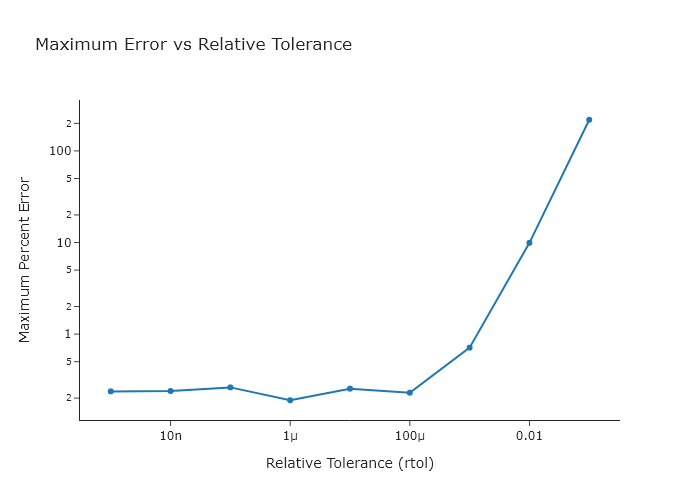

Exercise 0

Working from the code presented in Section \ref{Simulating_the_kinetics_of_one_elementary_reaction_using_scipy.solve_ivp}, use every option for the method keyword argument of scipy.solve_ivp() and compare the maximum error obtained. Try making a bar chart to compare these values, using Plotly. You can read the documentation in Chapter \ref{ch:plotly} for this, or use the quickBar() function out of codechembook.

import numpy as np
import scipy.integrate as spi
from plotly.graph_objects import Bar, Figure

# Define the differential equation
def FirstOrderDE(t, y, k):
    return -k * y

# Define the analytical solution
def analytical_solution(t, k, y0):
    return y0 * np.exp(-k * t)

# Simulation setup
y0 = 1.0
k = 1.0
time_span = [0, 10]
methods = ['RK45', 'RK23', 'Radau', 'BDF', 'LSODA']

# Store max errors
max_errors = []

# Evaluate each method
for method in methods:
    sol = spi.solve_ivp(FirstOrderDE, time_span, [y0], args=[k], method=method)
    y_exact = analytical_solution(sol.t, k, y0)
    percent_error = 100 * np.abs((sol.y[0] - y_exact) / y_exact)
    max_errors.append(np.max(percent_error))

# Plot using Plotly
fig = Figure(data=[
    Bar(x=methods, y=max_errors)
])
fig.update_layout(
    title='Maximum Percent Error by Method',
    xaxis_title='Method',
    yaxis_title='Max % Error',
    template='simple_white'
)
fig.show('png')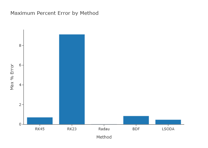

Simulating multi-step reaction mechanisms using scipy.solve ivp

Exercise 2

Using the code presented Section \ref{Simulating_multi-step_reaction_mechanisms_using_scipy.solve_ivp}. Adjust the reaction rates so that:

$[C]$ never levels off By the time $k_3 = 8e-1$, the concentration of C will not appear to level off.
Three of the traces appear to meet at a single point. _When k = [5e1, 0.8e1, 7e-1] the traces for B, cat, and X will appear to meet. _

Exercise 2

Using the code presented in Section \ref{Simulating_multi-step_reaction_mechanisms_using_scipy.solve_ivp}, adjust the initial concentrations so that:

There is only a single local maximum for $[X]$ Using y0 = [.1, .1, 0.2, 0.1, 0.0, 0.0] # concetrations (mM) [A, B, cat, X, Y, C] will result in this.
The bound catalyst is above a concentration of 0.5M for most of the time. Keeping the starting values all the same as in the book, but changing the value of \[X\] to be above 0.5 will result in this.

Exercise 2

Change the code in Section \ref{Simulating_multi-step_reaction_mechanisms_using_scipy.solve_ivp} so that the results are plotted versus $\ln(t)$. This makes it easier to focus on the early timepoints.

'''
A code to numerically solve a reaction mechanism that is irreversible but
has two intermediates using solve_ivp from scipy.integrate
    Written by: Ben Lear and Chris Johnson (authors@codechembook.com)
    v1.0.0 - 250217 - initial version
'''
import scipy.integrate as spi
from codechembook.quickPlots import quickScatter

# First we need to define a function containing our differential rate laws.
def TwoIntermediatesDE(t, y, k):
    '''
    Differential rate laws for a catalytic reaction with two intermediates:
    A + cat ->(k1) X
    X + B ->(k2) Y
    Y ->(k3) C + cat
    
    REQUIRED PARAMETERS:
    t (float):         the cutrent time in the simulation.  
                       Not explicitly used but needed by solve_ivp
    y (list of float): the current concentration
    k (list of float): the rate
    
    RETURNS:
    (list of float): rate of change of concentration in the order of y
    '''
    A, B, cat, X, Y, C = y # unpack concentrations to convenient variables
    k1, k2, k3 = k # unpack rates
    
    dAdt   = -k1 * A * cat
    dBdt   = -k2 * X * B
    dcatdt = -k1 * A * cat + k3 * Y
    dXdt   = k1 * A * cat - k2 * X * B
    dYdt   = k2 * X * B - k3 * Y
    dCdt   = k3 * Y
    
    return [dAdt, dBdt, dcatdt, dXdt, dYdt, dCdt]

# Set up initial conditions and simulation parameters
y0 = [1.0, 1.0, 0.2, 0.0, 0.0, 0.0] # concetrations (mM) [A, B, cat, X, Y, C]
k = [5e1, 1e1, 5e0]                 # rate (1/s)
time = [0, 10]                      # simulation start and end times (s)

# Invoke solve_ivp and store the result object
solution = spi.solve_ivp(TwoIntermediatesDE, time, y0, args = [k])

# Plot the results
fig = quickScatter(x = solution.t, # need a list of six identical time axes
             y = solution.y, 
             name = ['[A]', '[B]', '[cat]', '[X]', '[Y]', '[C]'],
             xlabel = 'Time (s)',
             ylabel = 'Concentration (mM)', 
             output = None)

fig.update_xaxes(type = "log")
fig.show("png")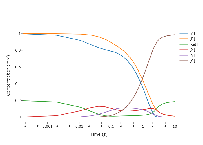

Comprehensive exercises

Exercise 5

It is often difficult to work second order processes, like:

\hspace{3em}$A + B \rightarrow C$

because the reaction progress depends strongly on both [A] and [B] (one of which may be hard to measure). Instead, you can work in excess [A] or [B] and make the “pseudo-first order approximation" to remove the explicit dependence of the differential rate law on its concentration. If, say, A is in excess, then [A] will not change much during the reaction, and can be approximated as a constant. Thus, we reduce:

\hspace{3em} $\frac{d[A]}{dt} = -k[A][B]$; \hspace{3em} $\frac{d[B]}{dt} = -k[A][B]$; \hspace{3em} $\frac{d[C]}{dt} = k[A][B]$;

\hspace{3em}to

\hspace{3em} $\frac{d[A]}{dt} = -\kappa[B]$; \hspace{3em} $\frac{d[B]}{dt} = -\kappa[B]$; \hspace{3em} $\frac{d[C]}{dt} = \kappa[B]$;

\hspace{3em} where

\hspace{3em} $\kappa = k[A]$

It is a good idea to figure out how much excess you need for the pseudo-first order approximation to hold. While this could be done analytically, it is quick and still quite accurate to do numerically. To do this, we will run several trials with increasing excess of A and track how the difference between the two solutions changes. To proceed:

Write scripts that model the second order and the pseudo-first order reactions.
Convert these codes into functions that take as arguments the initial concentrations, rates, and reaction times and return the solution object from solve_ivp()l
Write another script that creates a list of initial concentrations of A, starting with $[A]_0 = [B]_0$ and increasing logarithmically to $[A]_0 = 100 \times [B]_0$, and then solves both reactions for the same conditions.
For each condition, compute the sum of squared differences between the second order and pseudo-first order solutions for $[C](t)$. Note that because you are probably using an adaptive step size solver, the time points you get back by default will not be the same between the two reactions. Instead, you will need to use the tspan keyword to specify common time points. A good idea would be to make sure you are specifying time points that are no farther apart than the smallest gap between times in any simulation.
Plot the difference versus the ratio of concentrations for each time point. Identify the region of applicability for the pseudo-first order approximation.

import numpy as np
from scipy.integrate import solve_ivp
from plotly.subplots import make_subplots
import plotly.graph_objects as go

# Constants and setup
k = 1.0
B0 = 1.0
t_end = 10
t_eval = np.linspace(0, t_end, 500)
ratios = np.logspace(0, 2, 50)  # [A]_0 / [B]_0 from 1x to 100x

# Reaction definitions
def second_order(t, y):
    A, B, C = y
    rate = k * A * B
    return [-rate, -rate, rate]

def pseudo_first_order(t, y, kappa):
    B, C = y
    return [-kappa * B, kappa * B]

# Storage
ssd_list = []
representative_idx = 20  # Index to show full [C](t) comparison
C_full_plot = None
C_pseudo_plot = None
time_plot = None
diff_plot = None

# Compute
for i, ratio in enumerate(ratios):
    A0 = ratio * B0
    y0_full = [A0, B0, 0.0]
    sol_full = solve_ivp(second_order, [0, t_end], y0_full, t_eval=t_eval)

    kappa = k * A0
    y0_pseudo = [B0, 0.0]
    sol_pseudo = solve_ivp(pseudo_first_order, [0, t_end], y0_pseudo, args=(kappa,), t_eval=t_eval)

    C_full = sol_full.y[2]
    C_pseudo = sol_pseudo.y[1]
    ssd = np.sum((C_full - C_pseudo) ** 2)
    ssd_list.append(ssd)

    if i == representative_idx:
        time_plot = t_eval
        C_full_plot = C_full
        C_pseudo_plot = C_pseudo
        diff_plot = np.abs(C_full - C_pseudo)

# === Plotting with Plotly ===
fig = make_subplots(rows=3, cols=1,
                    shared_xaxes=False,
                    subplot_titles=[
                        "Sum of Squared Differences vs. [A]₀/[B]₀",
                        f"[C](t) Comparison at [A]₀ = {ratios[representative_idx]:.1f} × [B]₀",
                        "Absolute Difference in [C](t)"
                    ])

# 1. SSD vs. ratio
fig.add_trace(go.Scatter(
    x=ratios,
    y=ssd_list,
    mode='lines+markers',
    name='SSD vs ratio',
    line=dict(color='grey'),
    marker=dict(color='grey')
), row=1, col=1)

fig.update_xaxes(type='log', title='[A]₀ / [B]₀', row=1, col=1)
fig.update_yaxes(type='log', title='Sum of Squared Differences', row=1, col=1)

# 2. [C](t) comparison
fig.add_trace(go.Scatter(
    x=time_plot,
    y=C_full_plot,
    mode='lines',
    name='Second-order',
    line=dict(color='black')
), row=2, col=1)

fig.add_trace(go.Scatter(
    x=time_plot,
    y=C_pseudo_plot,
    mode='lines',
    name='Pseudo-first',
    line=dict(color='red')
), row=2, col=1)

fig.update_xaxes(title='Time', row=2, col=1)
fig.update_yaxes(title='[C](t)', row=2, col=1)

# 3. Difference over time
fig.add_trace(go.Scatter(
    x=time_plot,
    y=diff_plot,
    mode='lines',
    name='|ΔC|',
    line=dict(color='blue')
), row=3, col=1)

fig.update_xaxes(title='Time', row=3, col=1)
fig.update_yaxes(title='|[C]ₛₑcₒₙd - [C]ₚₛₑᵤ𝒹ₒ|', row=3, col=1)

fig.update_layout(
    height=900,
    width=800,
    title_text="Pseudo-First Order Approximation Analysis",
    showlegend=False
)

fig.show("png")

Exercise 6

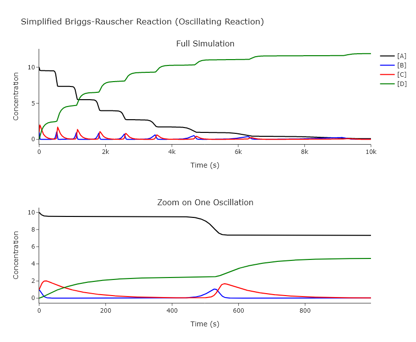
The iodine clock reaction is a classic chemistry demonstration. Look up a demonstration on YouTube if you’re not familiar. Accurately modeling it is complex, but a simplified model can be created using the Briggs-Rauscher reaction:

\hspace{3em} $\ce{A + B \overset{k_1}{->} 2 B}$

\hspace{3em} $\ce{B + C \overset{k_2}{->} 2 C}$

\hspace{3em} $\ce{C \overset{k_3}{->} D}$

Modify our ODE solving code to work on this system. Good starting points are initial concentrations $[A]_0 = 10$, $[B]_0 = 1$, $[C]_0 = 1$, $[D]_0 = 0$, $k_1 = 0.005$, $k_2 = 0.1$, $k_3 = 0.01$, and $t_{max} = 10000$. Change the initial concentrations and rates one at a time. Provide plots that show how all concentrations change with time, both for the full time range and one oscillation. Explain how this reaction works, particularly how it can oscillate even though all the reactions are forward only. Show the behavior at several limits in the rates and initial concentrations, particularly where the system no longer oscillates.

import numpy as np
from scipy.integrate import solve_ivp
import plotly.graph_objects as go
from plotly.subplots import make_subplots

# === Differential Equations ===
def br_oscillator(t, y, k):
    A, B, C, D = y
    k1, k2, k3 = k
    
    dAdt = -k1 * A * B
    dBdt = k1 * A * B - k2 * B * C
    dCdt = k2 * B * C - k3 * C
    dDdt = k3 * C
    
    return [dAdt, dBdt, dCdt, dDdt]

# === Initial conditions and parameters ===
y0 = [10.0, 1.0, 1.0, 0.0]        # [A], [B], [C], [D]
k = [0.005, 0.1, 0.01]            # [k1, k2, k3]
t_max = 10000
t_eval = np.linspace(0, t_max, 5000)

# === Solve ODEs ===
sol = solve_ivp(br_oscillator, [0, t_max], y0, args=(k,), t_eval=t_eval)

# === Plot with Plotly ===
fig = make_subplots(rows=2, cols=1,
                    shared_xaxes=False,
                    subplot_titles=["Full Simulation", "Zoom on One Oscillation"])

# Full time series
species = ['[A]', '[B]', '[C]', '[D]']
colors = ['black', 'blue', 'red', 'green']

for i, (name, color) in enumerate(zip(species, colors)):
    fig.add_trace(go.Scatter(
        x=sol.t, y=sol.y[i], mode='lines', name=name, line=dict(color=color)
    ), row=1, col=1)

# Zoom in: just show the first 1000 seconds (or modify as needed)
mask_zoom = sol.t <= 1000

for i, (name, color) in enumerate(zip(species, colors)):
    fig.add_trace(go.Scatter(
        x=sol.t[mask_zoom], y=sol.y[i][mask_zoom], mode='lines', showlegend=False, line=dict(color=color)
    ), row=2, col=1)

fig.update_layout(
    height=700,
    width=850,
    title="Simplified Briggs-Rauscher Reaction (Oscillating Reaction)",
    xaxis_title="Time (s)",
    yaxis_title="Concentration (mM)",
    template="simple_white"
)

fig.update_xaxes(title_text="Time (s)", row=1, col=1)
fig.update_xaxes(title_text="Time (s)", row=2, col=1)
fig.update_yaxes(title_text="Concentration", row=1, col=1)
fig.update_yaxes(title_text="Concentration", row=2, col=1)

fig.show()