Exercises
Targeted exercises
Getting yes/no answers to questions posed by comparison statements
Exercise 0
What do the following conditional expressions evaluate to (True or False)? First, write down what you think it should be before running the code, then run it to see if you are right. If you were wrong, explain what you did wrong. Suppose the following variables are already defined:
trial_number = 4;
pH = 2.53;
acid = 'HCl';
conc_stock = 1.0 # M
pH >= 2acid != 'HF'trial_number > 2pH > 1conc_stock / 1000 < 0.001acid == 'HF''H' in acid.
trial_number = 4
pH = 2.53
acid = 'HCl'
conc_stock = 1.0

print(pH >= 2)
print(acid != 'HF')
print(trial_number > 2)
print(pH > 1)
print(acid == 'HF')
print('H' in acid)
Exercise 1
Write a conditional expression to evaluate the following tests. Use the variable name given in parentheses for your answer. Define the following variables:
pKa = 7.6;
atomic_number = 19;
pH = 4.4;
atom_symbol = 'K';
solvent_name = 'Isopropanol';
formula = '(CH3)2CHOH';
solvent_polarity = 3.9`;
\textbf{example}: Is the $pK_a$ (pKa) less than 5.0?: pKa < 5.0
- Is the atomic number equal to 11?
- Is the pH at least 4 but less than 6?
- Is the atom symbol ‘K’
- Is the solvent ‘Methanol’ or ‘Acetonitrile’? (note: do this with a single comparison)
- Is the string ‘OH’ in ‘formula’? .
pKa = 7.6
atomic_number = 19
pH = 4.4
atom_symbol = 'K'
solvent_name = 'Isopropanol'
formula = '(CH3)2CHOH'
solvent_polarity = 3.9


print(atomic_number == 11)
print(4 <= pH <6)
print(atom_symbol == "K")
print(solvent_name in ["Methanol", "Acetonitrile"])
print("OH" in formula)
Exercise 2
For the dictionary of solvent properties created in Exercise 0 of Chapter 5, write a code that determines if an alcohol is in the dictionary by testing to see if 'ol' is in any of the keys. You can do this by getting a list of the keys using list(<dictionaryname>.keys()) and then iterating through that list, or by using for k in <dictionaryname>:
benzene = {
	"IUPAC" : "benzene",
	"MW" : 78.114, #g/mol
	"BP" : 80.1, # degrees C
	"rho" : 0.8765, #g/cm3
	}

cyclohexane = {
    "IUPAC": "cyclohexane",
    "MW": 84.16,       # g/mol
    "BP": 80.7,        # °C
    "rho": 0.7781,     # g/cm³
}

n_hexane = {
    "IUPAC": "hexane",
    "MW": 86.18,       # g/mol
    "BP": 68.7,        # °C
    "rho": 0.6603,     # g/cm³
}

toluene = {
    "IUPAC": "methylbenzene",
    "MW": 92.14,       # g/mol
    "BP": 110.6,       # °C
    "rho": 0.8669,     # g/cm³
}

methanol = {
    "IUPAC": "methanol",
    "MW": 32.04,       # g/mol
    "BP": 64.7,        # °C
    "rho": 0.7918,     # g/cm³
}

acetonitrile = {
    "IUPAC": "acetonitrile",
    "MW": 41.05,       # g/mol
    "BP": 81.6,        # °C
    "rho": 0.786,      # g/cm³
}

solvents = {
	"benzene": benzene,
	"cyclohexane" : cyclohexane,
	"n_hexane" : n_hexane,
	"toluene" : toluene,
	"methanol" : methanol,
	"acetonitrile" : acetonitrile,
	}

# check to see if "ol" in key...
for k in solvents:
    print(k, "has 'ol'?", "ol" in k)
Slicing arrays by values instead of indices using comparison expressions
Exercise 3
Create a sine wave with period of 1 with an $x$-axis that goes from 0 to 20 with 100 elements. Make a plot of this sine wave where positive values are green and negative values are blue using slicing to produce two different $y$ arrays and two corresponding $x$ arrays that you can plot separately. If you set mode = "markers" when you add scatter traces, then you will not get a line at zero.
import numpy as np
from plotly.subplots import make_subplots

x = np.linspace(0, 4*np.pi, 1000)
y = np.sin(x)

pos_index = y>=0
neg_index = y<0

fig = make_subplots()
fig.add_scatter(x = x[pos_index], y = y[pos_index],
                mode = "markers", marker = dict(color = "green"),
                showlegend = False)
fig.add_scatter(x = x[neg_index], y = y[neg_index],
                mode = "markers", marker = dict(color = "blue"),
                showlegend = False)

fig.show("png")
Slicing based on multiple conditions using and and or
Exercise 4
What do the following conditional expressions evaluate to (True or False)? First, write down what you think it should be before running the code, then run it to see if you are right. If you were wrong, explain what you did wrong. Suppose the following variables are already defined:
trial_number = 4;
pH = 2.53;
acid = 'HCl';
conc_stock = 1.0 # M;
pH >= 2 and pH < 7acid != 'HF' and acid != 'HBr'trial_number > 2 and acid != 'HCl'pH > 1 and pH < 7acid == 'HCl' or acid == 'HF'(pH > 2 and acid == 'HF') or (pH > 3 and acid == 'HCl').
trial_number = 4
pH = 2.53
acid = 'HCl'
conc_stock = 1.0

print(pH >= 2 and pH < 7)
print(acid != 'HF' and acid != 'HBr')
print(trial_number > 2 and acid != 'HCl')
print(pH > 1 and pH < 7)
print(acid == 'HCl' or acid == 'HF')
print((pH > 2 and acid == 'HF') or (pH > 3 and acid == 'HCl'))
Exercise 5
Write a conditional expression to evaluate the following tests. Use the variable name given in parentheses for your answer. Define the following variables:
pKa = 7.6;
atomic_number = 19;
pH = 4.4;
atom_symbol = 'K';
solvent_name = 'Isopropanol';
formula = '(CH3)2CHOH';
solvent_polarity = 3.9`;
- Is the solvent anything other than ‘Toluene’ or ‘Hexanes’ and is the polarity less than 5?
- Is the pH greater than 4 and the $pK_a$ greater than 4?
- Does the formula contain a methyl group and an alcohol group?
- Is the atom potassium and the pH less than 2? .
pKa = 7.6
atomic_number = 19
pH = 4.4
atom_symbol = 'K'
solvent_name = 'Isopropanol'
formula = '(CH3)2CHOH'
solvent_polarity = 3.9

print(solvent_name != "Toluene" and solvent_name != "Hexanes" and solvent_polarity < 5)
print(pH > 4 and pKa > 4)
print("CH3" in formula and "OH" in formula)
print(atom_symbol == 'K' and pH < 2)
Visualizing fit results using codechembook.quickPlots.plotFit
Exercise 6
Modify the code from Chapter 5 to use the plotFit() function from codechembook and confirm that it works.
'''
A script to fit a calibration experiment to a line, starting wtih the UV/vis
spectra
    Requires: .csv files with col 1 as wavelength and col 2 as intensity
               filenames should contain the concentration after an '_'
    Written by: Ben Lear and Chris Johnson (authors@codechembook.com)
    v1.0.0 - 250204 - initial version
'''
import numpy as np
from lmfit.models import LinearModel
from plotly.subplots import make_subplots
from codechembook.quickTools import quickSelectFolder
import codechembook.symbols as cs
from codechembook.quickPlots import plotFit

# identify the files you wish to plot and the place you want to save them at
print('Select the folder with the calibration UVvis files.')
filenames = sorted(quickSelectFolder().glob('*csv'))

# Ask the user what wavelength to use for calibration
l_max = float(input('What is the position of the feature of interest? '))

# Loop through the file names, read the files, and extract the data into lists
conc, absorb = [], [] # empty lists that will hold concentrations and absorbances
for f in filenames:
    conc.append(float(f.stem.split('_')[1])) # get concentration from file name and add to list
    temp_x, temp_y = np.genfromtxt(f, unpack = True, delimiter=',', skip_header = 1) # read file
    l_max_index = np.argmin(abs(temp_x - l_max)) # Find index of x data point closest to l_max
    absorb.append(temp_y[l_max_index]) # get the closest absorbance value and add to list

# Set up and perform a linear fit to the calibration data
lin_mod = LinearModel() # create an instance of the linear model object
pars = lin_mod.guess(absorb, x=conc) # have lmfit guess at initial values
result = lin_mod.fit(absorb, pars, x=conc) # fit using these initial values
print(result.fit_report()) # print out the results of the fit

# Print out the molar absorptivity
print(f'The molar absorptivity is {result.params['slope'].value / 1:5.2f} {cs.math.plusminus} {result.params['slope'].stderr:4.2f} M{cs.typography.sup_minus}{cs.typography.sup_1}cm{cs.typography.sup_minus}{cs.typography.sup_1}')

# Construct a plot with two subplots.  Pane 1 contains the best fit and data, pane 2 the residual
fig = plotFit(result, output = None, residual = True)

# Create annotation for the slope and intercept values and uncertainties as a string
annotation_string = f'''
slope = {result.params['slope'].value:.2e} {cs.math.plusminus} {result.params['slope'].stderr:.2e}<br>
intercept = {result.params['intercept'].value:.2e} {cs.math.plusminus} {result.params['intercept'].stderr:.2e}<br>
R{cs.typography.sup_2} = {result.rsquared:.3f}'''

fig.add_annotation(text = annotation_string,
                   x = np.min(result.userkws['x']), y = result.data[-1],
                   xanchor = 'left', yanchor = 'top', align = 'left',
                   showarrow = False, )

# Create annotation for the extinction coefficient and uncertainty
fig.add_annotation(text = f'{cs.greek.epsilon} = {result.params['slope'].value:5.2f} {cs.math.plusminus} {result.params['slope'].stderr:4.2f} M<sup>-1</sup>cm<sup>-1</sup>',
                   x = np.max(result.userkws['x']), y = result.data[0],
                   xanchor = 'right', yanchor = 'top', align = 'right',
                   showarrow = False, )

# Format the axes and the plot, then show it
fig.update_xaxes(title = 'concentration /M')
fig.update_yaxes(title = f'absorbance @ {l_max} nm', row = 1, col = 1)
fig.update_yaxes(title = 'residual absorbance', row = 2, col = 1)
fig.update_layout(template = 'simple_white')
fig.show('png')
Learning to use libraries by reading documentation
Exercise 7
Read the documentation for the plotFit() function and make plots for the code from the end of the chapter but with the following changes:
- Confidence intervals of 95%.
- Hide the components of the fit.
- Show the residual but scale it to the same scale as the main plot. .
'''
Fit data to multiple gaussian components and a linear background
    Requires: a .csv file with col 1 as wavelength and col 2 as intensity
    Written by: Ben Lear and Chris Johnson (authors@codechembook.com)
    v1.0.0 - 250207 - initial version
'''
import numpy as np
from lmfit.models import LinearModel, GaussianModel
from codechembook.quickPlots import plotFit
import codechembook.symbols as cs
from codechembook.quickTools import quickOpenFilename, quickPopupMessage

# Ask the user for the filename containing the data to analyze
quickPopupMessage(message = 'Select the file 0.001.csv')
file = quickOpenFilename(filetypes = 'CSV Files, *.csv')

# Read the file and unpack into arrays
wavelength, absorbance = np.genfromtxt(file, skip_header=1, unpack = True, delimiter=',')

# Set the upper and lower wavelength limits of the region of the spectrum to analyze
lowerlim, upperlim = 450, 750

# Slice data to only include the region of interest
trimmed_wavelength = wavelength[(wavelength >= lowerlim) & (wavelength < upperlim)]
trimmed_absorbance = absorbance[(wavelength >= lowerlim) & (wavelength < upperlim)]

# Construct a composite model and include initial guesses
final_mod = LinearModel(prefix='lin_') # start with a linear model and add more later
pars = final_mod.guess(trimmed_absorbance, x=trimmed_wavelength) # get guesses for linear coefficients
c_guesses = [532, 580, 625] # initial guesses for centers
s_guess = 10 # initial guess for widths
a_guess = 20 # initial guess for amplitudes
for i, c in enumerate(c_guesses): # loop through each peak to add corresponding gaussian component
    gauss = GaussianModel(prefix=f'g{i+1}_') # create temporary gaussiam model
    pars.update(gauss.make_params(center=dict(value=c), # set initial guesses for parameters
                               amplitude=dict(value=a_guess, min = 0),
                               sigma=dict(value=s_guess, min = 0, max = 25)))
    final_mod = final_mod + gauss # add each peak to the overall model

# Fit the model to the data and store the results
result = final_mod.fit(trimmed_absorbance, pars, x=trimmed_wavelength)

# Create a plot of the fit results but don't show it yet
plot = plotFit(result,
               residual = "scaled",
               components = False,
               xlabel = 'wavelength /nm',
               ylabel = 'intensity',
               confidence = 95,
               output = None)

plot.show('png') # show the final plot
Exercise 7
Sometimes you may want to have a string representation of a whole array. Read the documentation for numpy.array2string() and use it to create a string that represents the sin wave from Exercise 3 rounded to the nearest tenth. Make sure that the output does not contain any newline (\n) characters using keywords for the function.
import numpy as np

x = np.linspace(0, 4*np.pi, 1000)
y = np.sin(x)

np.array2string(y, max_line_width=1e6, precision=1)
Combining lmfit models
Exercise 9
There are times where the behavior of a system is best described by the sum of the equations for two lines. For instance you could have a reaction mechanism with distinct rate-determining steps, where one dominates at early times and another takes over later. You might also encounter this in thermal expansion of multi-phase materials. Though the model needed to describe such behavior is simple, it would be somewhat challenging to use it in a fit within Excel and extracted parameter estimates and their uncertainties. Write the code to produce a lmfit model that is made up of two linear models.
import numpy as np
from lmfit.models import LinearModel

# Define two linear models for two regions
model1 = LinearModel(prefix='m1_')
model2 = LinearModel(prefix='m2_')

# Combine them
composite_model = model1 + model2
Accessing the number of times a loop has iterated using enumerate
Exercise 10
If you had two lists [ 1, 2, 3] and [4, 5, 6, 7] use enumerate() to add the first list to the first three elements of the second list.
l1 = [1, 2, 3]
l2 = [4, 5, 6, 7]

for i, n in enumerate(l1):
	l2[i] = l2[i] + n

print(l2)
Exercise 11
For the list [5, 1, 9, -3] construct a new list using a nested for loop. This new list must hold only the unique 6 pairwise products.
pairwise = []
l = [5, 1, 9 , -3]

for i, n in enumerate(l):
	for m in l[:i]:
		pairwise.append(n*m)

print(pairwise)
Comprehensive exercises
Exercise 12
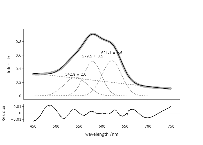
It is a good idea to check how robust the fitting results are—that is, how different can your initial guesses be, and still get the same final fit values. The fit for the Gaussians used in the final code of this chapter has three kinds of initial guesses: those for the position of the Gaussian, the intensity of the Gaussian, and the width of the Gaussian. For each of these parameter groups:
- Change the initial guesses in a way that you still get the same final fit (within the errors of the parameters).
- Change the initial guesses in a way that you do not get the same final fit (within the errors of the parameters).
- Comment on how robust this fitting seems to you.
The Original:

If you change the guess for the longest wavelength to as long as 670, you get the same.
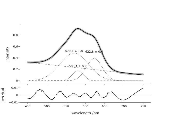
 But if you change to 675, you get.
 Considering this, it seems unreasonable to guess the longest wavelength to be 675, so this fit seems fairly robust against reasonable guesses for this longest wavelength. You can explore the effects changing the guesses for other parameters.
Exercise 13
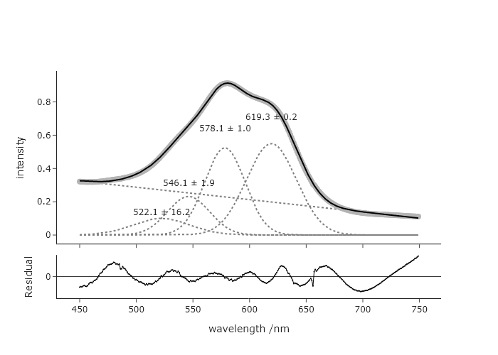
Using the final code for the chapter, modify this so that there is no upper bound on the Gaussian width parameter. When you run this version, do you get a different result? If so, discuss why you might, or might not use this upper bound, and if you could justify using it.
The result when you remove the upper bound:
This suggests that either the restriction to 3 features is not correct, that the band is made up of these three bands with very different widths, or that one needs to impose a chemically reasonable shape on the fit.
Exercise 14
You think that there may be a small 4$^{th}$ Gaussian contribution in the data that was fit in the final code of this chapter, and it looks like it would be around 500 nm. Change the code to allow for fitting of this 4$^{th}$ peak. Discuss the results of this new fit with respect to the one that was presented at the end of the chapter.
Adding a new peak is as simple as adding a new guess within the c list. However, in order to get a reasonable fit, one needs to impose a minimum width that is more than 0. This fit is with a minimum of 10. The need to introduce a new restriction maybe suggests that this is not as good a fit as before. However,, the original AIC was -3108 and the new AIC is -3383, which suggests that the 4th peak is adding meaningful information.
Exercise 14
Modify the code we produced at the end of this chapter to add annotations that label the peaks of the actual signal (instead of the Gaussian components) with the best fitting peak centers. The annotation should include an arrow that points to this exact position in the data, which can be accomplished directly in the add_annotation() method of the Plotly figure.
Pay attention to how the y-position is found, and the setting of the arrow appearing and the offset along y.
'''
Fit data to multiple gaussian components and a linear background
    Requires: a .csv file with col 1 as wavelength and col 2 as intensity
    Written by: Ben Lear and Chris Johnson (authors@codechembook.com)
    v1.0.0 - 250207 - initial version
'''
import numpy as np
from lmfit.models import LinearModel, GaussianModel
from codechembook.quickPlots import plotFit
import codechembook.symbols as cs
from codechembook.quickTools import quickOpenFilename, quickPopupMessage

# Ask the user for the filename containing the data to analyze
#quickPopupMessage(message = 'Select the file 0.001.csv')
#file = quickOpenFilename(filetypes = 'CSV Files, *.csv')
file = "C:/Users/benle/Documents/GitHub/Coding-for-Chemists/Distribution/Catalyst/Titration/UVvis/0.001.csv"

# Read the file and unpack into arrays
wavelength, absorbance = np.genfromtxt(file, skip_header=1, unpack = True, delimiter=',')

# Set the upper and lower wavelength limits of the region of the spectrum to analyze
lowerlim, upperlim = 450, 750

# Slice data to only include the region of interest
trimmed_wavelength = wavelength[(wavelength >= lowerlim) & (wavelength < upperlim)]
trimmed_absorbance = absorbance[(wavelength >= lowerlim) & (wavelength < upperlim)]

# Construct a composite model and include initial guesses
final_mod = LinearModel(prefix='lin_') # start with a linear model and add more later
pars = final_mod.guess(trimmed_absorbance, x=trimmed_wavelength) # get guesses for linear coefficients
c_guesses = [ 550, 580, 650] # initial guesses for centers
s_guess = 10 # initial guess for widths
a_guess = 20 # initial guess for amplitudes
for i, c in enumerate(c_guesses): # loop through each peak to add corresponding gaussian component
    gauss = GaussianModel(prefix=f'g{i+1}_') # create temporary gaussiam model
    pars.update(gauss.make_params(center=dict(value=c), # set initial guesses for parameters
                               amplitude=dict(value=a_guess, min = 0),
                               sigma=dict(value=s_guess, min = 10, max = 25)))
    final_mod = final_mod + gauss # add each peak to the overall model

# Fit the model to the data and store the results
result = final_mod.fit(trimmed_absorbance, pars, x=trimmed_wavelength)

# Create a plot of the fit results but don't show it yet
plot = plotFit(result, residual = True, components = True, xlabel = 'wavelength /nm', ylabel = 'intensity', output = None)

# Add best fitting value for the center of each gaussian component as annotations
for i in range(1, len(c_guesses)+1): # loop through components and add annotations with centers
    plot.add_annotation(text = f"{result.params[f'g{i}_center'].value:.1f} {cs.math.plusminus} {result.params[f'g{i}_center'].stderr:.1f}",
                        x = result.params[f'g{i}_center'].value,
                        y = result.best_fit[np.argmin(abs(np.array(trimmed_wavelength) - result.params[f'g{i}_center'].value))],
                        ax = 0, ay = -50,
                        showarrow = True)

plot.show('png') # show the final plot
Exercise 15
It is technically not a good idea to fit bands to Gaussian functions when your $x$-axis is in wavelength. You should really be working in an energy unit, since the effects that give rise to peak shapes depend on energy rather than wavelength, and intensities in the two are related by a Jacobian transformation (see Exercise 28 of Chapter 2 for details). Rewrite the code at the end of this chapter to first convert the $x$-axis to electron volts (eV), then perform the fit in those units. Note: you will need to convert the guesses as well to get a good start. How do the results compare between these two approaches?
import numpy as np
from lmfit.models import LinearModel, GaussianModel
from codechembook.quickPlots import plotFit
import codechembook.symbols as cs
from codechembook.quickTools import quickOpenFilename, quickPopupMessage
# Ask the user for the filename containing the data to analyze
quickPopupMessage(message='Select the file 0.001.csv')
file = quickOpenFilename(filetypes='CSV Files, *.csv')
#%%
# Read the file and unpack into arrays
wavelength_nm, absorbance = np.genfromtxt(file, skip_header=1, unpack=True, delimiter=',')
# Define wavelength limits and convert to energy limits (eV)
lowerlim_nm, upperlim_nm = 450, 750
eV_conversion = lambda wl: 1240 / wl
energy_eV = eV_conversion(wavelength_nm)
# Slice data based on wavelength range, then reverse for increasing energy order
mask = (wavelength_nm >= lowerlim_nm) & (wavelength_nm < upperlim_nm)
trimmed_energy = energy_eV[mask][::-1]
trimmed_absorbance = absorbance[mask][::-1]
# Apply Jacobian correction: A(E) = A(λ) * dλ/dE = A(λ) * 1240 / E^2
trimmed_absorbance = trimmed_absorbance * (1240 / trimmed_energy**2)
# Construct a composite model and include initial guesses (converted to eV)
final_mod = LinearModel(prefix='lin_')
pars = final_mod.guess(trimmed_absorbance, x=trimmed_energy)
# Initial guesses (in nm) converted to eV
c_guesses_nm = [520, 580, 625]
c_guesses_eV = [1240 / nm for nm in c_guesses_nm]
s_guess_nm = 10
s_guess_eV = np.mean([(1240 / (nm - s_guess_nm)) - (1240 / nm) for nm in c_guesses_nm]) # approx conversion
a_guess = 20
for i, c in enumerate(c_guesses_eV):
gauss = GaussianModel(prefix=f'g{i+1}_')
pars.update(gauss.make_params(center=dict(value=c),
amplitude=dict(value=a_guess, min=0),
sigma=dict(value=s_guess_eV, min=0, max=20))) # eV scale for sigma
final_mod = final_mod + gauss
# Fit the model
result = final_mod.fit(trimmed_absorbance, pars, x=trimmed_energy)
# Plot
plot = plotFit(result, residual=True, components=True,
xlabel='energy /eV', ylabel='intensity (Jacob. corrected)', output=None)
# Annotate Gaussian peak centers
for i in range(1, len(c_guesses_eV)+1):
center = result.params[f'g{i}_center'].value
error = result.params[f'g{i}_center'].stderr
amplitude = result.params[f'g{i}_amplitude'].value
sigma = result.params[f'g{i}_sigma'].value
height = amplitude / (sigma * np.sqrt(2 * np.pi))
plot.add_annotation(
text=f'{center:.2f} {cs.math.plusminus} {error:.2f} eV',
x=center,
y=i * 0.04 + height,
showarrow=False
)
plot.show('png')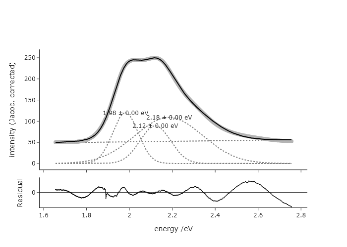 This fit is very different, at least in terms of widths and intensities. The reduced chi squared for this is ~1.4, while for the fit in terms of wavelength is ~2.9, suggesting the fit in terms of eV is more accurate.
Exercise 15
In Chapter 3, we plotted many of the same spectra that we fit here. Generate a script that automatically fits each of these spectra and produces a single Plotly plot for each spectrum that was fit, each in its own subplot. Do not include the residuals. You may find that this code eventually ‘breaks.’ This is likely be because the guesses for parameters are no longer good places to start, for later titration points.
'''
Fit data to multiple gaussian components and a linear background
Requires: a .csv file with col 1 as wavelength and col 2 as intensity
Written by: Ben Lear and Chris Johnson (authors@codechembook.com)
v1.0.0 - 250207 - initial version
'''
import numpy as np
from lmfit.models import LinearModel, GaussianModel
import codechembook.symbols as cs
from codechembook.quickTools import quickOpenFilenames, quickPopupMessage
from plotly.subplots import make_subplots
# Ask the user for the filename containing the data to analyze
quickPopupMessage(message = 'select all the data files')
files = quickOpenFilenames(filetypes = 'CSV Files, *.csv')
#%%
# Create a plot of the fit results but don't show it yet
plot = make_subplots(rows = len(files), cols = 1)
for p, file in enumerate(files):
# Read the file and unpack into arrays
wavelength, absorbance = np.genfromtxt(file, skip_header=1, unpack = True, delimiter=',')
# Set the upper and lower wavelength limits of the region of the spectrum to analyze
lowerlim, upperlim = 450, 750
# Slice data to only include the region of interest
trimmed_wavelength = wavelength[(wavelength >= lowerlim) & (wavelength < upperlim)]
trimmed_absorbance = absorbance[(wavelength >= lowerlim) & (wavelength < upperlim)]
# Construct a composite model and include initial guesses
final_mod = LinearModel(prefix='lin_') # start with a linear model and add more later
pars = final_mod.guess(trimmed_absorbance, x=trimmed_wavelength) # get guesses for linear coefficients
c_guesses = [532, 580, 625] # initial guesses for centers
s_guess = 10 # initial guess for widths
a_guess = 20 # initial guess for amplitudes
for i, c in enumerate(c_guesses): # loop through each peak to add corresponding gaussian component
gauss = GaussianModel(prefix=f'g{i+1}_') # create temporary gaussiam model
pars.update(gauss.make_params(center=dict(value=c), # set initial guesses for parameters
amplitude=dict(value=a_guess, min = 0),
sigma=dict(value=s_guess, min = 0, max = 25)))
final_mod = final_mod + gauss # add each peak to the overall model
try:
# Fit the model to the data and store the results
result = final_mod.fit(trimmed_absorbance, pars, x=trimmed_wavelength)
plot.add_scatter(x = trimmed_wavelength, y = trimmed_absorbance, line = dict(color = 'grey', width = 4), row = p+1, col = 1)
plot.add_scatter(x = trimmed_wavelength, y = result.best_fit, row = p+1, col = 1)
# Add best fitting value for the center of each gaussian component as annotations
for i in range(1, len(c_guesses)+1): # loop through components and add annotations with centers
plot.add_annotation(text = f"{result.params[f'g{i}_center'].value:.1f} {cs.math.plusminus} {result.params[f'g{i}_center'].stderr:.1f}",
x = result.params[f'g{i}_center'].value,
y = i*.04 + result.params[f'g{i}_amplitude'].value / (result.params[f'g{i}_sigma'].value * np.sqrt(2*np.pi)),
showarrow = False,
row = i+1, col = 1)
except:
plot.add_annotation(text = "fit failed",
x = 600, y = 0.5,
row = p+ 1, col = 1)
plot.update_layout(height = 1800)
plot.show('browser') # show the final plot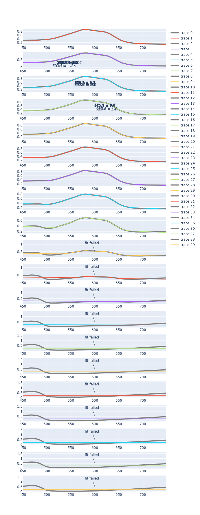 _To fix this, you would perhaps need to implement a new fit window, when the first fit fails. _