Exercises
Targeted exercises
Prompting the user for information using input
Exercise 0
Using the dictionary of solvent properties that you made in Exercise 0 from Chapter 4, write a code that asks the user for a solvent, then asks the user for a property, and then prints a sentence that tells the user the value of that property for the solvent they chose.
benzene = {
	"IUPAC" : "benzene",
	"MW" : 78.114, #g/mol
	"BP" : 80.1, # degrees C
	"rho" : 0.8765, #g/cm3
	}

cyclohexane = {
    "IUPAC": "cyclohexane",
    "MW": 84.16,       # g/mol
    "BP": 80.7,        # °C
    "rho": 0.7781,     # g/cm³
}

n_hexane = {
    "IUPAC": "hexane",
    "MW": 86.18,       # g/mol
    "BP": 68.7,        # °C
    "rho": 0.6603,     # g/cm³
}

toluene = {
    "IUPAC": "methylbenzene",
    "MW": 92.14,       # g/mol
    "BP": 110.6,       # °C
    "rho": 0.8669,     # g/cm³
}

methanol = {
    "IUPAC": "methanol",
    "MW": 32.04,       # g/mol
    "BP": 64.7,        # °C
    "rho": 0.7918,     # g/cm³
}

acetonitrile = {
    "IUPAC": "acetonitrile",
    "MW": 41.05,       # g/mol
    "BP": 81.6,        # °C
    "rho": 0.786,      # g/cm³
}

solvents = {
	"benzene": benzene,
	"cyclohexane" : cyclohexane,
	"n_hexane" : n_hexane,
	"toluene" : toluene,
	"methanol" : methanol,
	"acetonitrile" : acetonitrile,
	}

# get dictionary

sol = input("What solvent are you interested in?")
prop = input("What property are you interested in?")

print("The", prop, "of", sol, "is", solvents[sol][prop])
Turning numeral characters into numbers
Exercise 1
Modify the script from the end of Chapter 0 so that it asks the user for the concentration of HCl, ionic strength, and concentration of the catalyst, then performs the calculation and outputs results in the same way as before.
def calcPlateVols(conc_cat, conc_HCl, I, vol_final = 1):

    # Define our stock solutions
    conc_stock_cat = 0.1 # M
    conc_stock_HCl = 6 # M
    conc_stock_NaCl = 3 # M

    # Calculate the volumes needed
    vol_cat = conc_cat / conc_stock_cat * vol_final
    vol_HCl = conc_HCl / conc_stock_HCl * vol_final
    vol_NaCl = (I - conc_HCl) / conc_stock_NaCl * vol_final

    # Calculate the water needed to make up 1 mL
    vol_water = vol_final - vol_cat - vol_HCl - vol_NaCl

    print('[ ] catalyst solution (mL)\n', vol_cat)
    print('[ ] HCl (mL)\n', vol_HCl)
    print('[ ] NaCl (mL)\n', vol_NaCl)
    print('[ ] water (mL)\n', vol_water)

conc_HCl = float(input("What is the concentration of HCl in M? "))
conc_cat = float(input("What is the concentration of the catalyst in M? "))
I = float(input("What is the desired final ionic strength in M? "))

calcPlateVols(conc_cat, conc_HCl, I)
Inserting calculation results into strings using f-strings
Exercise 2
Using f-strings and the print() function, output a grammatically correct sentence that expresses the following (perform the math, if necessary, and write out the result to the user in plain English including units). For each item, you can use a single line of code to accomplish this:
- The number of moles of water in 14.7 g.
- The density of toluene in g/mL.
- The number of mL in one gallon.
- 72.5 degrees Fahrenheit in Celsius.
print(f"The number of moles of water in 14.7 grams is {14.7 / 18.015} mol.")
print(f"The density of toluene is approximately {0.8669} g/mL.")
print(f"There are approximately {128 * 29.5735} milliliters in one gallon.")
print(f"72.5 degrees Fahrenheit is equivalent to {(72.5 - 32) * 5 / 9} degrees Celsius.")
Formatting the representation of numbers in strings
Exercise 3
In two lines of code, define the variable specified and print the following statement using f-strings to display the value of the variable, with units. Remember that Python uses banker’s rounding:
- Given
normal_temp = 293.15, print ‘Normal temperature is 293.1 K.’ - Given
vol = 1.672834e-3, print ‘The volume is 1.673 mL.’ - Given
conc_NaCl = 0.0043782, print ‘[NaCl] = 4.38 mM.’ - Given
ethane_CC_bond_length = 153.5, print ‘Ethane’s C-C bond is 0.153 nm.’
normal_temp = 293.15
print(f"Normal temperature is {normal_temp:.1f} K.")

vol = 1.672834e-3
print(f"The volume is {vol*1e3:.3f} mL.")

conc_NaCl = 0.0043782
print(f"[NaCl] = {conc_NaCl * 1000:.2f} mM.")

ethane_CC_bond_length = 153.5
print(f"Ethane’s C-C bond is {ethane_CC_bond_length / 1000:.3f} nm.")
Generating symbols that aren’t on your keyboard using codechembook.symbols
Exercise 4
Create the f-strings that produce the following text, using the codechembook.symbols module to generate special characters:
- $\lambda_{\textrm{max}}$
- 3.27 $\mu$L.
- $\ce{[CH3CH2COO–]}$ = 5.14 mM.
- N$_2$ + 3H$_2$ → 2NH$_3$.
- The C=C bond length of ethylene is 1.33 \AA.
- For $p$ orbitals, $\ell = 1$.
from codechembook import symbols as s

vol = 3.27
print(f"{vol} {s.greek.mu}L.")

conc = 5.14
print(f"{('[CH3CH2COO–]')} = {conc} mM.")

print(f"{('N2')} + 3{('H2')} {s.chem.rxn_arrow_right} 2{('NH3')}.")

bond_length = 1.33
print(f"The CC bond length of ethylene is {bond_length} {s.chem.Angstrom}.")

print(f"For p orbitals, {s.script.l} = 1.")
Producing formatted chemical formulas using texttt codechembook.quickHTMLFormula()
Exercise 6
Repeat Exercise 11 from Chapter 4, using codechembook.quickTools.quickHTMLFormula().
from plotly.subplots import make_subplots
from codechembook.quickTools import quickFormula
fig = make_subplots()

fig.add_annotation(text = f'''</br>
                   {quickFormula('CH3')}</br>
                   {quickFormula('CH3CH2OH')}</br>
                   {quickFormula('(C8H17)4N', 1)}</br>
                   {quickFormula('C6H6')}</br>
''',
	showarrow = False
    )

fig.update_xaxes(visible = False)
fig.update_yaxes(visible = False)
fig.update_layout(template = "simple_white")
fig.show("png")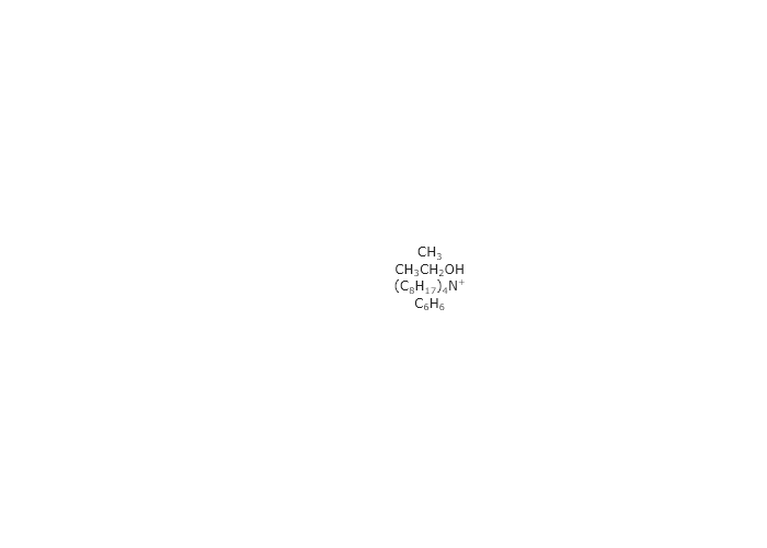
Finding paths to files in folders using glob
Exercise 5
Using the .glob() method of pathlib Path objects:
- Get a list of all the files in your Downloads folder.
- Sort the list of files you just made.
- Using
len(), print the number of .pdf files you have in your Downloads folder.
from pathlib import Path

downloads = Path("C:/Users/authors/Downloads")
pdf_files = sorted(downloads.glob("*.pdf"))
print(f"You have {len(pdf_files)} PDF files in your Downloads folder.")
You will, of course, need to change the Path to be the one to your own downloads.
Dividing a string into multiple substrings with split
Exercise 6
You have an irritating instrument that outputs data in text files interspersed in sentences. For instance, it will produce a string that goes like this:
“at 1.58 seconds, conc = 40.2 mM;at 3.24 seconds, conc = 78.2 mM;at 4.98 seconds, conc = 119.4 mM;at 6.02 seconds, conc = 154.7 mM”
You want to plot concentration versus time, but you first need to process this string. Using the .split() method for strings, write a script that:
- Breaks apart the above string to extract the times and concentrations
- Processes these times and concentrations them into Numpy arrays.
- Plots these arrays with proper axis labels.
- Makes no assumptions about how many data points there are.
import numpy as np
from plotly.subplots import make_subplots

data_str = (
    "at 1.58 seconds, conc = 40.2 mM;at 3.24 seconds, conc = 78.2 mM;at 4.98 seconds, conc = 119.4 mM;at 6.02 seconds, conc = 154.7 mM"
)

# Split into individual measurements
measurements = data_str.split(";")
#print(measurements)

# Prepare lists for time and concentration
times = []
concs = []

for measurement in measurements:
    text_time, text_conc = measurement.split(",")
    times.append(float(text_time.split(" ")[1]))
    concs.append(float(text_conc.split(" ")[3])) # because of leading space

# Convert to numpy arrays
time_array = np.array(times)
conc_array = np.array(concs)

# Plot
fig = make_subplots()
fig.add_scatter(x=time_array, y=conc_array, mode='markers+lines')
fig.update_xaxes(title = "Time /s")
fig.update_yaxes(title = "Concentration /mM")
fig.show("png")
Finding the element closest to a given number in a Numpy array
Exercise 7
If you used the approach we demonstrated in this chapter to find a number closest to a target number, what happens if there are two numbers that are equally close to the target number? In this case, the first element will be returned, but not the second.
Exercise 7
Write code that will take a Numpy array and find a number in it, closest to some target number. Write this code such that, if there are two (or more) numbers that are equally close to the target number, you identify the smallest number.
import numpy as np

array = np.array([3, 5, -3, -5])


def get_closest_smallest(reference, array):
	found_value = None
	subtracted = abs(array) - reference
	min_value = np.min(subtracted)
	for i, value in subtracted:
		if value == min_value:
			if found_value is None:
				found_value = array[i]
			else: # already have a value
				if array[i] < found_value:
					found_value = array[i]
	return found_value

get_closest_smallest(0, array)
Fitting models to data with lmfit
Exercise 9
You have measured the equilibrium constant for a chemical reaction at multiple temperatures. You wish to use a Van’t Hoff plot to determine $\Delta H$ and $\Delta S$ for the reaction. The equation for this is $\ln(K_{eq}) = -\frac{\Delta H}{RT} + \frac{\Delta S}{R}$. Thinking about this proceedure, you realize that this form of the equation was historically used because it produces a linear relationship between $\ln(K_{eq})$ and $\frac{1}{T}$ and this was simpler to fit in the time before computers. However, both of these transformations can significantly change the values of the parameters that are estimated by the fit. So, what you should actually do is plot $K_{eq}$ versus $T$ and fit that plot. Write the equation you would use as the model for this fitting and identify the independent variable, the dependent variable, the parameters you would adjust in a fit, and any constants that would not change in the fit.
$K_{eq}(T) = e^{-\frac{\Delta H}{RT} + \frac{\Delta S}{R}}$ _In this equation, the independent variable is $T$, the dependent variable is $K_{EQ}$, the parameters are $\Delta H$ and $\Delta S$, and R is a constant. _
Analyzing fit results in lmfit
Exercise 13
Use the Spyder IDE’s variable explorer orprint(vars(result)) to inspect the fitResult object created by the final code in this chapter. You will find that it is presented as if it had some dictionary structure. The ‘keys’ are the attributes of the result object and are used to access the associated ‘values.’ For instance, if you wanted to find the R$^2$ value of the fit, you could use result.rsquared, which should return something like 0.9994452445068337. Find the attributes for the following elements:
- The best-fitting values
- Their uncertainties
- Whether the fit was aborted
- The model used
- $\chi^2$
| Element | Access Method | Description |
|---|---|---|
| Best-fitting values | fitResults.best_values |
Dictionary of best-fit parameter values. |
| Uncertainties | fitResults.params['param_name'].stderr |
Standard error of a specific parameter. |
| Fit aborted status | fitResults.success |
Boolean indicating if the fit was successful. |
| Model used | fitResults.model |
The model instance used for fitting. |
| R² (coefficient of determination) | Not directly available; see explanation below. | Measures how well the model explains the data. |
| χ² (chi-square) | fitResults.chisqr |
Sum of squared residuals; lower values indicate a better fit. |
Building figures with multiple subplots in Plotly
Exercise 11
Make a figure with two subplots, one on top and one on bottom, in which the top plot is the first spectrum from our titration series in Chapter 3 and the bottom plot is the last one.
import numpy as np
from plotly.subplots import make_subplots
from codechembook.quickTools import quickOpenFilenames

# First, we need the names of the files that we want to plot
# Ask the user to select the files and then sort the resulting list
data_files = quickOpenFilenames(filetypes = 'CSV files, *.csv')
sorted_data_files = sorted(data_files)

# Next, we will process one file at a time and add it to the plot
titration_endpoints = make_subplots(rows = 2, cols = 1) # start a blank plotly figure object
startx, starty np.genfromtxt(sorted_files[0],
        delimiter = ',', skip_header = 1, unpack = True)
titration_endpoints.add_scatter(x = startx, y = starty, row = 1, col = 1)

endx, endy = np.genfromtxt(sorted_files[-1],
        delimiter = ',', skip_header = 1, unpack = True)
titration_endpoints.add_scatter(x = endx, y = endy, row = 2, col = 1)

titration_series.show("png")
titration_series.write_image('titration.png', width = 3*300, height = 2*300)
Exercise 12
Make a figure with four subplots, in two rows and two columns, in which the top left plot is the first spectrum from our titration series in Chapter 3, the bottom right is the last spectrum, the top right is the first spectrum minus the last spectrum, and the bottom left is the last spectrum minus the first spectrum.
import numpy as np
from plotly.subplots import make_subplots
from codechembook.quickTools import quickOpenFilenames

# First, we need the names of the files that we want to plot
# Ask the user to select the files and then sort the resulting list
data_files = quickOpenFilenames(filetypes = 'CSV files, *.csv')
sorted_data_files = sorted(data_files)
#%%
# Next, we will process one file at a time and add it to the plot
titration_endpoints = make_subplots(rows = 2, cols = 2) # start a blank plotly figure object
startx, starty = np.genfromtxt(sorted_data_files[0],
        delimiter = ',', skip_header = 1, unpack = True)
titration_endpoints.add_scatter(x = startx, y = starty, row = 1, col = 1)

endx, endy = np.genfromtxt(sorted_data_files[-1],
        delimiter = ',', skip_header = 1, unpack = True)
titration_endpoints.add_scatter(x = endx, y = endy, row = 2, col = 2)

titration_endpoints.add_scatter(x = startx, y = starty - endy, row = 1, col = 2) #top right

titration_endpoints.add_scatter(x = startx, y = endy - starty, row = 2, col = 1) # bottom left

titration_endpoints.show("png")
titration_series.write_image('titration.png', width = 3*300, height = 2*300)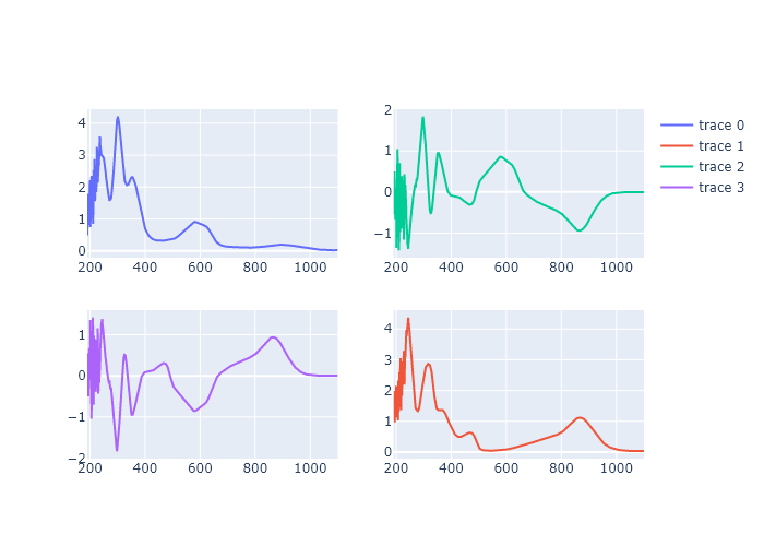
Comprehensive exercises
Exercise 16
In this chapter, we introduced a function that makes it easy to identify multiple files on your computer: quickSelectFolder(). This will be nice to use when you don’t know where the file is located, or when you are choosing different files each time you run your script. However, there will be times when you simply want to use the same file over and over—for instance when you are developing and testing a code. In these cases, it can be much faster to provide the path to the file in the script. Modify the final code in this chapter, replacing the quickSelectFolder() function with a line that creates a Path object with the absolute path to the folder and on which you use the glob() method. Verify this works, and describe when you might prefer this approach over the use of quickSelectFolder().
'''
A script to fit a calibration experiment to a line, starting wtih the UV/vis
spectra
    Requires: .csv files with col 1 as wavelength and col 2 as intensity
               filenames should contain the concentration after an '_'
    Written by: Ben Lear and Chris Johnson (authors@codechembook.com)
    v1.0.0 - 250204 - initial version
'''
import numpy as np
from lmfit.models import LinearModel
from plotly.subplots import make_subplots
from codechembook.quickTools import quickSelectFolder
import codechembook.symbols as cs
from pathlib import Path # need a path object for glob

# identify the files you wish to plot and the place you want to save them at
print('Select the folder with the calibration UVvis files.')
filenames = sorted(Path("C:/Users/benle/Documents/GitHub/Coding-for-Chemists/Distribution/Catalyst/Extinction").glob('*csv'))

# Ask the user what wavelength to use for calibration
l_max = float(input('What is the position of the feature of interest? '))

# Loop through the file names, read the files, and extract the data into lists
conc, absorb = [], [] # empty lists that will hold concentrations and absorbances
for f in filenames:
    conc.append(float(f.stem.split('_')[1])) # get concentration from file name and add to list
    temp_x, temp_y = np.genfromtxt(f, unpack = True, delimiter=',', skip_header = 1) # read file
    l_max_index = np.argmin(abs(temp_x - l_max)) # Find index of x data point closest to l_max
    absorb.append(temp_y[l_max_index]) # get the closest absorbance value and add to list

# Set up and perform a linear fit to the calibration data
lin_mod = LinearModel() # create an instance of the linear model object
pars = lin_mod.guess(absorb, x=conc) # have lmfit guess at initial values
result = lin_mod.fit(absorb, pars, x=conc) # fit using these initial values
print(result.fit_report()) # print out the results of the fit

# Print out the molar absorptivity
print(f'The molar absorptivity is {result.params['slope'].value / 1:5.2f} {cs.math.plusminus} {result.params['slope'].stderr:4.2f} M{cs.typography.sup_minus}{cs.typography.sup_1}cm{cs.typography.sup_minus}{cs.typography.sup_1}')

# Construct a plot with two subplots.  Pane 1 contains the best fit and data, pane 2 the residual
fig = make_subplots(rows = 2, cols = 1) # make a blank figure object that has two subplots

# Add trace objects for the best fit, the data, and the residualto the plot
fig.add_scatter(x = result.userkws['x'], y = result.best_fit, mode = 'lines', showlegend=False, row = 1, col = 1)
fig.add_scatter(x = result.userkws['x'], y = result.data, mode = 'markers', showlegend=False, row =1, col = 1)
fig.add_scatter(x = result.userkws['x'], y = -1*result.residual, showlegend=False, row = 2, col = 1)

# Create annotation for the slope and intercept values and uncertainties as a string
annotation_string = f'''
slope = {result.params['slope'].value:.2e} {cs.math.plusminus} {result.params['slope'].stderr:.2e}<br>
intercept = {result.params['intercept'].value:.2e} {cs.math.plusminus} {result.params['intercept'].stderr:.2e}<br>
R{cs.typography.sup_2} = {result.rsquared:.3f}'''

fig.add_annotation(text = annotation_string,
                   x = np.min(result.userkws['x']), y = result.data[-1],
                   xanchor = 'left', yanchor = 'top', align = 'left',
                   showarrow = False, )

# Create annotation for the extinction coefficient and uncertainty
fig.add_annotation(text = f'{cs.greek.epsilon} = {result.params['slope'].value:5.2f} {cs.math.plusminus} {result.params['slope'].stderr:4.2f} M<sup>-1</sup>cm<sup>-1</sup>',
                   x = np.max(result.userkws['x']), y = result.data[0],
                   xanchor = 'right', yanchor = 'top', align = 'right',
                   showarrow = False, )

# Format the axes and the plot, then show it
fig.update_xaxes(title = 'concentration /M')
fig.update_yaxes(title = f'absorbance @ {l_max} nm', row = 1, col = 1)
fig.update_yaxes(title = 'residual absorbance', row = 2, col = 1)
fig.update_layout(template = 'simple_white')
fig.show('png')
The answer will depend on your specific computer. This will be more useful anytime you are not changing the location each time you run the code, or when you can type out the location faster than finding the file/folder in a browser.
Exercise 17
You remember from analytical chemistry that there is a ‘linear regime’ for absorbance values. You wonder about the behavior in transmittance. Convert the values used in the final code of this chapter to transmittance, and fit that to a line, displaying the data, fit, and residual of the fit. If you use R$^2$ of 0.99 as a threshold for ‘good’ linearity, then how is this fit? .
'''
A script to fit a calibration experiment to a line, starting wtih the UV/vis
spectra
Requires: .csv files with col 1 as wavelength and col 2 as intensity
filenames should contain the concentration after an '_'
Written by: Ben Lear and Chris Johnson (authors@codechembook.com)
v1.0.0 - 250204 - initial version
'''
import numpy as np
from lmfit.models import LinearModel
from plotly.subplots import make_subplots
from codechembook.quickTools import quickSelectFolder
import codechembook.symbols as cs
from pathlib import Path # need a path object for glob
# identify the files you wish to plot and the place you want to save them at
print('Select the folder with the calibration UVvis files.')
filenames = sorted(Path("C:/Users/benle/Documents/GitHub/Coding-for-Chemists/Distribution/Catalyst/Extinction").glob('*csv'))
# Ask the user what wavelength to use for calibration
l_max = float(input('What is the position of the feature of interest? '))
# Loop through the file names, read the files, and extract the data into lists
conc, absorb = [], [] # empty lists that will hold concentrations and absorbances
for f in filenames:
conc.append(float(f.stem.split('_')[1])) # get concentration from file name and add to list
temp_x, temp_y = np.genfromtxt(f, unpack = True, delimiter=',', skip_header = 1) # read file
l_max_index = np.argmin(abs(temp_x - l_max)) # Find index of x data point closest to l_max
absorb.append(temp_y[l_max_index]) # get the closest absorbance value and add to list
trans = 10**-np.array(absorb)# convert to transmittance
# Set up and perform a linear fit to the calibration data
lin_mod = LinearModel() # create an instance of the linear model object
pars = lin_mod.guess(trans, x=conc) # have lmfit guess at initial values
result = lin_mod.fit(trans, pars, x=conc) # fit using these initial values
print(result.fit_report()) # print out the results of the fit
# Print out the molar absorptivity
print(f'The molar absorptivity is {result.params['slope'].value / 1:5.2f} {cs.math.plusminus} {result.params['slope'].stderr:4.2f} M{cs.typography.sup_minus}{cs.typography.sup_1}cm{cs.typography.sup_minus}{cs.typography.sup_1}')
# Construct a plot with two subplots. Pane 1 contains the best fit and data, pane 2 the residual
fig = make_subplots(rows = 2, cols = 1) # make a blank figure object that has two subplots
# Add trace objects for the best fit, the data, and the residualto the plot
fig.add_scatter(x = result.userkws['x'], y = result.best_fit, mode = 'lines', showlegend=False, row = 1, col = 1)
fig.add_scatter(x = result.userkws['x'], y = result.data, mode = 'markers', showlegend=False, row =1, col = 1)
fig.add_scatter(x = result.userkws['x'], y = -1*result.residual, showlegend=False, row = 2, col = 1)
# Create annotation for the slope and intercept values and uncertainties as a string
annotation_string = f'''
slope = {result.params['slope'].value:.2e} {cs.math.plusminus} {result.params['slope'].stderr:.2e}<br>
intercept = {result.params['intercept'].value:.2e} {cs.math.plusminus} {result.params['intercept'].stderr:.2e}<br>
R{cs.typography.sup_2} = {result.rsquared:.3f}'''
fig.add_annotation(text = annotation_string,
x = np.min(result.userkws['x']), y = result.data[-1],
xanchor = 'left', yanchor = 'top', align = 'left',
showarrow = False, )
# Create annotation for the extinction coefficient and uncertainty
fig.add_annotation(text = f'{cs.greek.epsilon} = {result.params['slope'].value:5.2f} {cs.math.plusminus} {result.params['slope'].stderr:4.2f} M<sup>-1</sup>cm<sup>-1</sup>',
x = np.max(result.userkws['x']), y = result.data[0],
xanchor = 'right', yanchor = 'top', align = 'right',
showarrow = False, )
# Format the axes and the plot, then show it
fig.update_xaxes(title = 'concentration /M')
fig.update_yaxes(title = f'absorbance @ {l_max} nm', row = 1, col = 1)
fig.update_yaxes(title = 'residual absorbance', row = 2, col = 1)
fig.update_layout(template = 'simple_white')
fig.show('png')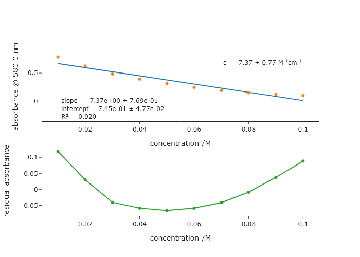 Looking at this plot, you can see that even at 580nm in the spectrum, the non-linearity of the transmittance is already obvious.
Exercise 18
It is common to fit models that depend exponentially on some value, like kinetics, by taking the natural log of the dependent variable and performing a linear fit instead of fitting the raw data to an exponential function:
\hspace{5em} $[A](t) = [A]_0\exp{-kt} \rightarrow \ln{\frac{[A](t)}{[A]_0}} = -kt$
In the absence of noise, these two approaches to fitting are equivalent. However, if your data is somewhat noisy, you can get different results from the two different approaches.
- Download the file ‘expfit.csv’ and save it to your class folder. This file has three columns: time (sec), exact concentration (M), and noisy concentration (M). Load the data and create new arrays containing the natural log of the concentrations. Then, fit both forms of the raw data to exponentials, and both forms of the natural log data to lines. Compare the rates that you get from the linear model to the exponential model for the exact and noisy cases. What do you notice? Make a table here of your results and include your code when you turn in the assignment.
- The above problem can be mostly remedied. Since LMFIT is basically trying to minimize $\chi^2$, which depends on the uncertainty of each point. In the data you’ve been given, the uncertainty of each point is the same ($\sigma$ = 0.0001). When you take the natural log of the $y$-values, you also have to compute new uncertainties in the logarithmic space, which are not all the same! Thus, not all points have equal weight when calculating $\chi^2$. LMFIT allows you to give each point a different weight using the weight keyword in
Model.fit()(check it out in the documentation. The weights should be $\frac{1}{\sigma_i^2}$ for each point. When you take the log, the new uncertainties $\sigma{'}_i^2$ in the logarithmic y axis can be computed by $\sigma{'}_i = \frac{\sigma_i}{y_i}$. Using this relationship, revise your code to do the linear fit with appropriate weights, and confirm that it makes the results more consistent. .
import numpy as np
from lmfit.models import LinearModel, ExponentialModel
from codechembook.quickPlots import plotFit

t, ylin, ylinnoise = np.genfromtxt('./Data/expfit.csv', delimiter = ',', skip_header = 1, unpack = True)
yln = np.log(ylin/ylin[0])
ylnnoise = np.log(ylinnoise/ylinnoise[0])

linearmodel = LinearModel()
linearparams = linearmodel.guess(yln, x = t)
linearresult = linearmodel.fit(yln, linearparams, x = t)
print(linearresult.best_values['slope'])

linearmodel_noise = LinearModel()
linearparams_noise = linearmodel.guess(ylnnoise, x = t)
linearresult_noise = linearmodel.fit(ylnnoise, linearparams_noise, x = t, weights = ylinnoise**2/1e-8)#1 / (ylnnoise + np.log(1e-2))**2)
print(linearresult_noise.best_values['slope'])

expmodel = ExponentialModel()
expparams = expmodel.guess(ylin, x = t)
expresult = expmodel.fit(ylin, expparams, x = t)
print(expresult.best_values['decay']**-1)

expmodel_noise = ExponentialModel()
expparams_noise = expmodel.guess(ylinnoise, x = t)
expresult_noise = expmodel.fit(ylinnoise, expparams_noise, x = t)
print(expresult_noise.best_values['decay']**-1)
Exercise 19
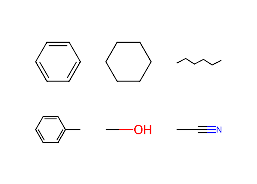
Using the solvent dictionary from Exercise 3 in Chapter 4, make a Plotly figure that has a grid of subplots equal to or greater than the number of solvents in that dictionary. Using RDKit, add a drawing of one solvent molecule to each subplot. It ok if you end up with blank subplots. In order to specify which subplot you are adding a figure to, you can use the xref=f"x{i}" and yref=f"y{i}" within the add_layout_image() method of the Plotly figure object. Here, i indicates the subplot number. Plotly counts subplots left to right, top to bottom (like you read English), and starts at the number 1.
from plotly.subplots import make_subplots
from rdkit import Chem
from rdkit.Chem import Draw
import base64

fig = make_subplots(2,3)

solvents_list = list(solvents.keys())

for i in range(3):
    for j in range(2):

        fig.update_xaxes(visible = False, range = [0,1], row = j+1, col = i+1)
        fig.update_yaxes(visible = False, range = [0,1], row = j+1, col = i+1)

        # Create an RDKit molecule object from a SMILES string
        mol = Chem.MolFromSmiles(solvents[solvents_list[i+3*j]]['smiles'])

        # Set options for drawing
        drawer = Draw.MolDraw2DSVG(100, 100) # create a canvas to draw on
        #drawer.drawOptions().setBackgroundColour((0, 0, 0, 0)) # the canvas color

        # Now that the options are set, we can process the molecule drawing
        drawer.DrawMolecule(mol) # create the drawing instructions
        drawer.FinishDrawing() # use the drawing instructions to make the drawing

        # Generate the SVG instructions then convert to a Base64-encoded data URI with a Plotly-required preamble
        svg = drawer.GetDrawingText().replace('svg:', '')
        svg_data_uri = f"data:image/svg+xml;base64,{base64.b64encode(svg.encode('utf-8')).decode('utf-8')}"


        fig.add_layout_image(
            dict(source=svg_data_uri,
                xref=f'x{i+3*j+1}', yref=f'y{i+3*j+1}', # references for coordinate origin
                x=0.5, y=0.5, # x- and y-coordinate position of the image
                xanchor='center', yanchor='middle',# alignment of image wrt x,y coords
                sizex=200, sizey=1)) # width and height of the image

    fig.update_layout(template = 'simple_white')
fig.show('png')