Exercises

Targeted exercises

Accessing items from dictionaries using keys

Exercise 0

Starting with the dictionary that you made in Exercise 22 of Chapter 3, print the following properties for the given solvent:

The boiling point of cyclohexane.
The density of toluene.
The IUPAC name of $n$-hexane.
The density of a mixture of 75% acetonitrile and 25% $n$-hexane (assume ideal behavior).

benzene = {
	"IUPAC" : "benzene",
	"MW" : 78.114, #g/mol
	"BP" : 80.1, # degrees C
	"rho" : 0.8765, #g/cm3
	}
	
cyclohexane = {
    "IUPAC": "cyclohexane",
    "MW": 84.16,       # g/mol
    "BP": 80.7,        # °C
    "rho": 0.7781,     # g/cm³
}

n_hexane = {
    "IUPAC": "hexane",
    "MW": 86.18,       # g/mol
    "BP": 68.7,        # °C
    "rho": 0.6603,     # g/cm³
}

toluene = {
    "IUPAC": "methylbenzene",
    "MW": 92.14,       # g/mol
    "BP": 110.6,       # °C
    "rho": 0.8669,     # g/cm³
}

methanol = {
    "IUPAC": "methanol",
    "MW": 32.04,       # g/mol
    "BP": 64.7,        # °C
    "rho": 0.7918,     # g/cm³
}

acetonitrile = {
    "IUPAC": "acetonitrile",
    "MW": 41.05,       # g/mol
    "BP": 81.6,        # °C
    "rho": 0.786,      # g/cm³
}

solvents = {
	"benzene": benzene,
	"cyclohexane" : cyclohexane,
	"n_hexane" : n_hexane,
	"toluene" : toluene,
	"methanol" : methanol,
	"acetonitrile" : acetonitrile,
	}

print(solvents["cyclohexane"]["BP"])
print(solvents['toluene']['rho'])
print(solvents['acetonitrile']['IUPAC'])
print(0.75*solvents['acetonitrile']['rho'] + 0.25*solvents["n_hexane"]["rho"])

Exercise 1

It can be useful to get a collection of the keys and values of a dictionary. If you have a dictionary, my_dict, you can get a list of the keys using list(my_dict.keys()) and a list of the values using list(my_dict.values()). Using this approach, print out all the keys and values for the dictionary in Exercise 1.

print(solvents.keys())

print(solvents.values())

Exercise 2

You can iterate over dictionary keys, using for key in my_dict: Using this approach, and the dictionary from exercise 0, develop a pair of nested for loops that will print out the string "the value <property value> is associated with the <property> of <solvent>", where “<property value>” is the dictionary values of each solvent dictionary, “<property>” is the key associated with the value, and “<solvent>” is the solvent under consideration. The last two will be keys of the dictionary.

for solvent in solvents:
	for property in solvents[solvent]:
		print("the value", solvents[solvent][property], "is associated with the", property, "of", solvent)

Describing chemical structures using SMILES

Exercise 3

Update the dictionary from Exercise 0 to include the SMILES strings of each solvent.

solvents["benzene"]["smiles"] = "c1ccccc1"
solvents["cyclohexane"]["smiles"] = "C1CCCCC1"
solvents["n_hexane"]["smiles"] = "CCCCCC"
solvents["toluene"]["smiles"] = "Cc1ccccc1"
solvents["methanol"]["smiles"] = "CO"
solvents["acetonitrile"]["smiles"] = "CC#N"

Drawing molecules with RDKit

Exercise 4

Using rdkit, create an image of the structure of each molecule in the dictionary from Exercise 0. If you use the updated version (Exercise 3), then you can simply access the SMILES from the dictionary.

from rdkit import Chem
from rdkit.Chem import Draw

for solvent in solvents:
	molecule = Chem.MolFromSmiles(solvents[solvent]["smiles"])
	Draw.ShowMol(molecule)

Using tuples to create unchangeable lists

Exercise 5

Using two different methods, make a tuple with the elements: 3, ‘frog’, 9.73, False, 6.02e23`

(3, 'frog', 9.73, False, 6.02e23)

tuple([3, 'frog', 9.73, False, 6.02e23])

Specifying colors using the rgb standard

Exercise 6

Make a dictionary of the rgb color designations for the following colors and assign it to a variable. Use the convention that the maximum for any given channel is 255.

Pure red.
Pure blue.
Pure green.
Pure cyan.
Pure purple.
Pure orange.
Black.
50% gray.

colors = {
"red": (255, 0, 0),
"blue": (0, 0, 255),
"green": (0, 255, 0),
"cyan": (0, 255, 255),
"purple": (255, 0, 255),
"orange": (255, 164, 0),
"black": (0, 0, 0),
"grey50": (127, 127, 127),
}

Exercise 6

Find the rgb color designations for the colors of your current school or a past school. Continue using the convention that the maximum value is 255. Penn State blue: Penn State White: (255, 255, 255),Stoney Brook Red: (255, 0, 0), Stony Brook black: (0, 0, 0)

Decoding data from binary files

Exercise 1

There are no Exercises for this section

Adding images to Plotly figures

Exercise 2

Find a picture of the logo of your current/past school, lab, or employer and add it to a blank Plotly plot. If you find a bitmap image file (e.g., .png, .jpg, .jpeg, etc.), you can use source = <path to image>, though you can also read the online documentation for Plotly to find out how to do so. Additionally, if you wish to hide the axes, you can supply the keyword/value visible=False in the update_xaxes() and update_yaxes() methods.

from plotly.subplots import make_subplots

fig = make_subplots()

# Add invisible scatter plot to define axis range
fig.add_scatter(x=[0, 1], y=[0, 1], mode="markers", marker_opacity=0)

# Add logo image
fig.update_layout(
    images=[dict(
        source="C:/Users/benle/Downloads/PSU LOGO.png",  # local image path
        xref="paper", yref="paper",
        x=0.5, y=0.5,
        sizex=0.5, sizey=0.5,
        xanchor="center", yanchor="middle",
        sizing="contain",
        layer="above"
    )],
)

fig.update_xaxes(visible = False)
fig.update_yaxes(visible = False)
fig.show("png")
fig.show("png")

_This solution highlights yet another way to format Plotly figures: we can supply lots of information as dictionaries in the update_layout() method.

Adding annotations to Plotly figures

Exercise 3

Starting with the final code from Chapter 2, add an arrow pointing to the highest peak in the spectrum. The arrow line should have a width of 2 pixels and be red. The annotation text should also be red and say “Measure here (<wavelenth> nm)”

'''
A program to plot one uv-vis spectrum from a .csv file
    Requires: a .csv file with col 1 as wavelength and col 2 as intensity    
    Written by: Ben Lear and Chris Johnson (authors@codechembook.com)
    v1.0.0 - 250131 - initial version
'''
import numpy as np # needed for genfromtxt()
from plotly.subplots import make_subplots # needed to plot
from codechembook.quickTools import quickOpenFilename

# Specify the name and place for data
data_file = quickOpenFilename()

# Import wavelength (nm) and absorbance to plot as a numpy array
x_data, y_data = np.genfromtxt(data_file,
    delimiter = ',',
    skip_header = 1,
    unpack = True)

# Construct the plot - here UVvis holds the figure object
UVvis = make_subplots() # make a figure object
UVvis.add_scatter(x = x_data, y = y_data, # make a scatter trace object
    mode = 'lines', # this ensures that we will only get lines and not markers
    showlegend = False) # this prevents a legend from being automatically created

# Format the figure
UVvis.update_yaxes(title = 'absorbance')
UVvis.update_xaxes(title = 'wavelength /nm', range = [270, 1100])
UVvis.update_layout(template = 'simple_white') # set the details for the appearance 

UVvis.add_annotation(text = "Measure here (580 nm)",
                     x = 580, y = 0.91,
                     arrowcolor = "red",
                     arrowwidth = 2, 
                     arrowhead = 2,
                     font = dict(color = "red"))

# Display the figure
UVvis.show('browser+png') # show an interactive plot and in the spyder Plots window

# Save the spectra using the input file name but replacing .csv with the image file form
UVvis.write_image(data_file.with_suffix('.svg')) # save in the same location as the data file
UVvis.write_image(data_file.with_suffix('.png')) # save in the same location as the data file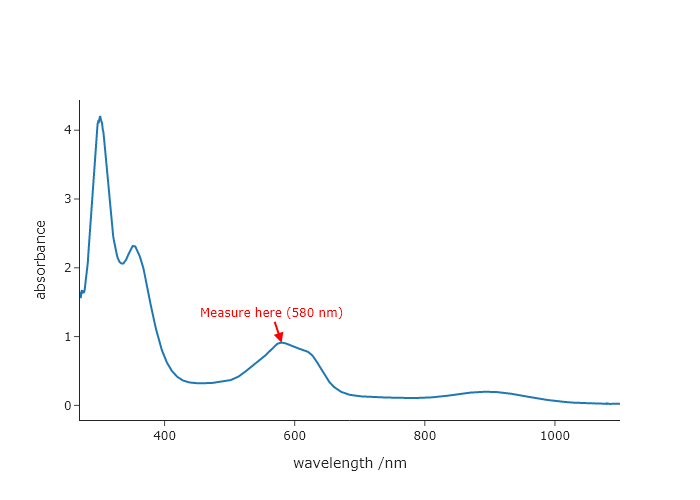

Formatting text in Plotly using HTML tags

Exercise 6

On a blank Plotly canvas, produce an annotation that is the properly formatted chemical formula for your five favorite molecules or complexes. This means using subscripts and superscripts.

from plotly.subplots import make_subplots

fig = make_subplots()

fig.add_annotation(text = '''</br>
CH<sub>3</sub>OH</br>
CH<sub>3</sub>CH<sub>2</sub>OH</br>
(C<sub>8</sub>H<sub>17</sub>)<sub>4</sub>N<sup>+</sup></br>
C<sub>6</sub>H<sub>6</sub></br>
''',
	showarrow = False,
    )
    
fig.update_xaxes(visible = False)
fig.update_yaxes(visible = False)
fig.update_layout(template = "simple_white")
fig.show("png")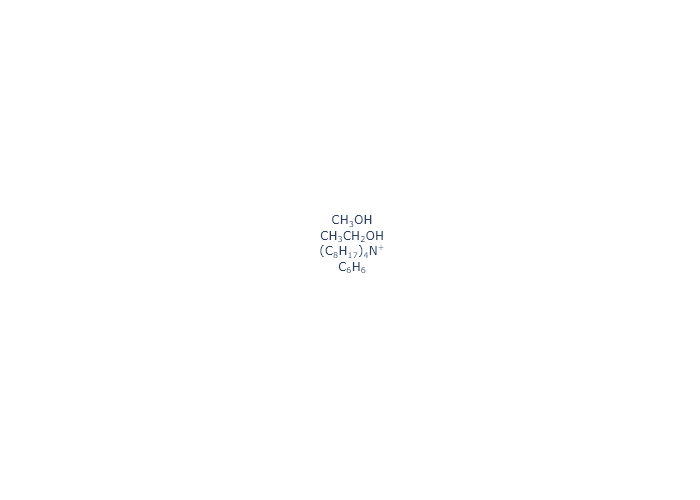

Producing HTML-formatted text quickly using codechembook.symbols

Exercise 5

Using codechembook.symbols.typesettingHTML, write out the following, using using proper formatting:

p$K_a$
$^2H$
$y = a\cdot x^2 + b\cdot x + c$

from codechembook.symbols import typesettingHTML as ts
from codechembook.symbols import math
print(f'p{ts.textit("K" + ts.textsub("a"))}')
print(f'{ts.textsup("2") + ts.textit("H")}')
print(f'{ts.textit("y = a" + math.cdot + "x" + ts.textsup("2") + "+ b"+ math.cdot + "x + c")}')

Exercise 6

Repeat Exercise 11 using the functions in codechembook.symbols.typesettingHTML. If you find formatting the chemical formulas frustrating, don’t worry, in the next chapter you will learn a better way to do this.

from plotly.subplots import make_subplots
from codechembook.symbols import typography
from codechembook.symbols.typesettingHTML import textsub as ts
from codechembook.symbols.typesettingHTML import textsup as tS

fig = make_subplots()

fig.add_annotation(text = f'''</br>
CH{ts('3')}OH</br>
CH{ts('3')}CH{ts('3')}OH</br>
(C{ts('8')}H{ts('17')}){ts('4')}N{tS('+')}</br>
C{ts('6')}H{ts('6')}</br>
''',
	showarrow = False
	)

fig.update_xaxes(visible = False)
fig.update_yaxes(visible = False)
fig.update_layout(template = "simple_white")
fig.show("png")

Generating sequences of numbers using range

Exercise 6

Create a list (not a generator) of integers from 0 to 10, including 10 using an expression that includes range().

list(range(0,11))

Exercise 6

Create a list (not a generator) of atomic numbers for the third row atoms using an expression that includes range().

list(range(3,11))

Exercise 6

Create a list (not a generator) of integers from 0 to -9, including -9 using an expression that includes range().

list(range(0,-10, -1))

Exercise 6

Create a tuple(not a generator) of integers between 0 and 100, including 100, spaced by 10, using an expression that includes range().

tuple(range(0,101,10))

Synchronizing iteration through multiple collections using zip

Exercise 10

You have the following two lists: one that holds the masses in grams of solvent in your sample ([0.567, 0.523, 0.263, 0.983, 0.634]), and one that holds the corresponding solvent name (['n-Hexane', 'Cyclohexane', 'Acetonitrile', 'Toluene', 'Benzene']). Write a single loop that prints out the volume of each solvent you used, including its name.

for g, s in zip([0.567, 0.523, 0.263, 0.983, 0.634], ['n-Hexane', 'Cyclohexane', 'Acetonitrile', 'Toluene', 'Benzene']):
	print("mass of", s, "is", g)

Specifying the result of function evaluation using the return keyword

Exercise 11

Make a function that computes the length of a list and returns it as an integer. Do not use len().

def get_len_list(lst):
	count = 0
	for item in lst:
		count = count + 1
	return len(count)

Exercise 11

Make a function that accepts two $x,y$-pairs and computes the slope and $y$-intercept associated with the line that would pass through both points and then and returns the value for the slope and the intercept.

def get_m_b(p1, p2):
	x1 = p1[0]
	x2 = p2[0]
	y1 = p1[1]
	y2 = p2[1]

	slope = (y2-y1)/(x2-x1)
	intercept = y1 - slope*x1
	return slope, intercept

Exercise 12

Modify the function from Exercise 19 to instead return a dictionary with two keys, slope and intercept.

def get_m_b(p1, p2):
	x1 = p1[0]
	x2 = p2[0]
	y1 = p1[1]
	y2 = p2[1]

	slope = (y2-y1)/(x2-x1)
	intercept = y1 - slope*x1
	return {"slope" : slope, "intercept" : intercept}

Describing how to use your functions in docstrings

Exercise 14

Make docstrings for the functions you created in Exercises 18–20. Include a description of the function’s purpose, the parameters it uses (with type and description), and the return value(s) (with type and description).

def get_len_list(lst):
    '''
    Parameters
    ----------
    lst : list, or really any iterable object

    Returns
    -------
    int: length of list

    '''
	count = 0
	for item in lst:
		count = count + 1
	return len(count)


def get_m_b(p1, p2):
    '''
    Parameters
    ----------
    p1 : list of x,y values for a point
    p2 : list of x,y values for a point

    Returns
    -------
    slope : float
    intercept : float
    '''
	x1 = p1[0]
	x2 = p2[0]
	y1 = p1[1]
	y2 = p2[1]

	slope = (y2-y1)/(x2-x1)
	intercept = y1 - slope*x1
	return slope, intercept

def get_m_b(p1, p2):
    '''
    Parameters
    ----------
    p1 : list of x,y values for a point
    p2 : list of x,y values for a point

    Returns
    -------
    dict : holds calculated slope and intercept, both as floats.

    '''
	x1 = p1[0]
	x2 = p2[0]
	y1 = p1[1]
	y2 = p2[1]

	slope = (y2-y1)/(x2-x1)
	intercept = y1 - slope*x1
	return {"slope" : slope, "intercept" : intercept}

Comprehensive exercises

Exercise 15

Starting with the dictionary from Exercise 3 of this chapter, write a code that will draw each chemical structure on a blank Plotly canvas. Arrange them in a grid. If you wish to hide the axes, you can supply the keyword/value visible=False in the update_xaxes() and update_yaxes() methods. In the chapter, we demonstrated how to display a svg image, if you would like use a png instead, you can use the function rdkit.Draw.MolToImage() and supply this the mol object.

This solution arranges them in a grid that is three columns wide.

from plotly.subplots import make_subplots
from rdkit import Chem
from rdkit.Chem import Draw
import base64

fig = make_subplots()
fig.update_xaxes(visible = False, range = [0,3])
fig.update_yaxes(visible = False, range = [0,2])

solvents_list = list(solvents.keys())

for i in range(6):

    y_index, x_index = divmod(i, 3)

    # Create an RDKit molecule object from a SMILES string
    mol = Chem.MolFromSmiles(solvents[solvents_list[i]]['smiles'])
    
    # Set options for drawing
    drawer = Draw.MolDraw2DSVG(100, 100) # create a canvas to draw on
    #drawer.drawOptions().setBackgroundColour((0, 0, 0, 0)) # the canvas color
    
    # Now that the options are set, we can process the molecule drawing
    drawer.DrawMolecule(mol) # create the drawing instructions
    drawer.FinishDrawing() # use the drawing instructions to make the drawing

    # Generate the SVG instructions then convert to a Base64-encoded data URI with a Plotly-required preamble
    svg = drawer.GetDrawingText().replace('svg:', '')
    svg_data_uri = f"data:image/svg+xml;base64,{base64.b64encode(svg.encode('utf-8')).decode('utf-8')}"
    
    
    fig.add_layout_image(
        dict(source=svg_data_uri,  
            xref='x', yref='y', # references for coordinate origin
            x=0.5+x_index, y=0.5+y_index, # x- and y-coordinate position of the image
            xanchor='center', yanchor='middle',# alignment of image wrt x,y coords
            sizex=200, sizey=1)) # width and height of the image
    
    fig.update_layout(template = 'simple_white')
fig.show('png')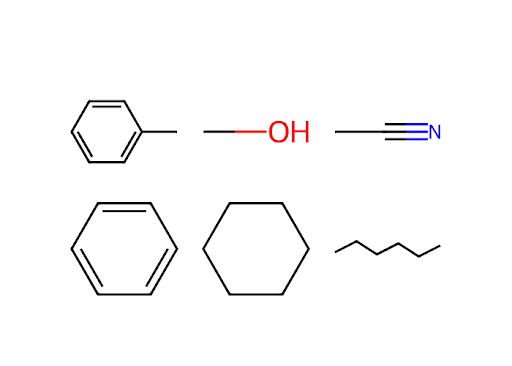

Exercise 16

You decide you want to include the formulas of the molecules in the final figure we created this chapter. Add them, using proper super scripting and subscripting for the formula and its charge. Make the formula text color also match the colors of the molecules they label using the font parameter of the add_annotation() method. If you need help, you can refer to the technical chapter on Plotly (Chapter \ref{ch:plotly}).

import numpy as np
from plotly.subplots import make_subplots
from codechembook.quickTools import quickOpenFilenames

# First, we need the names of the files that we want to plot
# Ask the user to select the files and then sort the resulting list
data_files = quickOpenFilenames(filetypes = 'CSV files, *.csv')
sorted_data_files = sorted(data_files)

# Next, we will process one file at a time and add it to the plot
titration_series = make_subplots() # start a blank plotly figure object

# Read the data in one file and add it as a scatter trace to the figure object
for file in sorted_data_files: # loop through the data files one at a time
    # Read the data and store it in temporary x and y variables
    x_data, y_data = np.genfromtxt(file,
        delimiter = ',', skip_header = 1, unpack = True)
    
    # Add data as scatter trace with formatted lines and exclude from legend
    titration_series.add_scatter(x = x_data, y = y_data,
                                 line = dict(color = 'gray', width = 1, dash = 'dot'),
                                 name = file.stem + ' eqs', showlegend=False)

# Adjust the appearance of only the first and last traces to highlight
titration_series.update_traces(selector = 0, # specify the initial trace
    line = dict(color = 'darkcyan', width = 2, dash = 'solid'), 
    showlegend = True, name = 'initial') 
    
titration_series.update_traces(selector = -1, # specify the final trace
    line = dict(color = 'darkred', width = 2, dash = 'solid'), 
    showlegend = True, name = 'final') 

# Move the initial trace to the end of the data, so that it is drawn on top
titration_series.data = titration_series.data[1:] + titration_series.data[:1]

# Format the plot area and then show it and then save it
titration_series.update_layout(template = 'simple_white')
titration_series.update_xaxes(title = 'wavelength /nm', range = [270, 1100])
titration_series.update_yaxes(title = 'absorbance', range = [0, 4.5])

from rdkit import Chem
from rdkit.Chem import Draw
from rdkit.Chem.Draw.MolDrawing import DrawingOptions
import base64
from codechembook.symbols.TypesettingHTML import textsup
from codechembook.quickTools import quickHTMLFormula

def make_mol_uri(smiles, color, bonds_wide, bonds_tall):
    '''
    Function to generate an svg of molecular drawing using rdkit and then return it in a format that is appropriate for inclusion in a Plotly figure object.

    REQUIRED PARAMETERS
    smiles (string):  Valid chemical smiles string.
    color (tuple):    Color designated in the rgb format.
    bonds_wide (int): Specifies how many bonds wide the structure is
    bonds_tall (int): Specifies how many bonds tall the structure is 

    RETURNS
    (bytes): Uri of the image for use in Plotly.
    '''
    # Create an RDKit molecule object from a SMILES string
    mol = Chem.MolFromSmiles(smiles)
    
    # Create a dictionary that defines the color of all atoms (here, the same)
    for key in range(1, 119):  # 119 is exclusive, so it goes up to 118
        DrawingOptions.elemDict[key] = color
    
    # Set options for drawing
    drawer = Draw.MolDraw2DSVG(50*bonds_wide, 50*bonds_tall) # create a canvas to draw on
    drawer.drawOptions().updateAtomPalette(DrawingOptions.elemDict) # the colors of atoms
    drawer.drawOptions().setBackgroundColour((0, 0, 0, 0)) # the canvas color
    
    # Now that the options are set, we can process the molecule drawing
    drawer.DrawMolecule(mol) # create the drawing instructions
    drawer.FinishDrawing() # use the drawing instructions to make the drawing

    # Generate the SVG instructions then convert to a Base64-encoded data URI with a Plotly-required preamble
    svg = drawer.GetDrawingText().replace('svg:', '')
    svg_data_uri = f"data:image/svg+xml;base64,{base64.b64encode(svg.encode('utf-8')).decode('utf-8')}"
    
    return svg_data_uri # return the binary code for the image
   
# Define the chemical formulas of the species 
base_formula = 'Ni(C4H2N2S2)2'
acid_formula = 'Ni(C4H2N2S2)2H'

# Define the charges of the species
base_charge = 0
acid_charge = 1

# Define the SMILES string for the base and acid species
base_smiles = 'C1(N=CC=N2)=C2O[Ni]3(O1)OC4=NC=CN=C4O3'
acid_smiles = '[H][N+]1=C2O[Ni]3(OC2=NC=C1)OC4=NC=CN=C4O3'

# Define colors for the base and acid species
base_color = (0, 139/255, 139/255) # dark cyan
acid_color = (139/255, 0, 0) # dark red

# Need a different way to define the colors for the plotly annotations
base_color_anno = 'darkcyan'
acid_color_anno = 'darkred'

# Loop through both molecules and create their respective images
for species, color, position, formula, charge, color_anno in zip(
        [base_smiles, acid_smiles], # the SMILES strings
        [base_color, acid_color], # the colors
        [580, 870], # the positions of the images on the plot area
        [base_formula, acid_formula], # the formulas of the species
        [base_charge, acid_charge], # the charges of the species
        [base_color_anno, acid_color_anno]):
    
    # Add image to plot
    titration_series.add_layout_image(
        dict(source=make_mol_uri(species, color, bonds_wide = 8, bonds_tall = 3),  
            xref='x', yref='y', # references for coordinate origin
            x=position, y=2.45, # x- and y-coordinate position of the image
            xanchor='center', yanchor='top',# alignment of image wrt x,y coords
            sizex=200, sizey=1)) # width and height of the image
    titration_series.add_annotation(
        dict(text = quickHTMLFormula(base_formula, charge = base_charge), font = dict(color = color_anno)),
        xref = 'x', yref = 'y',
        x = position, y = 2.65,
        xanchor = 'center', yanchor = 'middle',
        showarrow = False)
        
# Add an arrow to denote the reaction
titration_series.add_annotation(
    dict(ax = 680, ay = 2, # arrow start coordinates
    x = 770, y = 2, # arrow end coordinates
    axref = 'x', ayref = 'y', xref = 'x', yref = 'y', # references for coordinates
    showarrow = True, arrowhead = 1, arrowwidth = 1.5, arrowcolor = 'grey')) # arrow format

# Add H+ label
titration_series.add_annotation(
    dict(text = 'H' + textsup('+'), font = dict(color = 'grey'),
    xref = 'x', yref = 'y', # references for coordinate origin
    x = (770+680)/2, y = 2, # x- and y-coordinate position of the image
    xanchor = 'center', yanchor = 'bottom', # location of text box wrt position
    showarrow = False))      # we want no arrow associated with this annotation

# eliminate the legend entries for all traces
titration_series.update_traces(showlegend = False)

# Now output the plot
titration_series.show('png+browser')
titration_series.write_image('titration.png', width = 6*300, height = 4*300)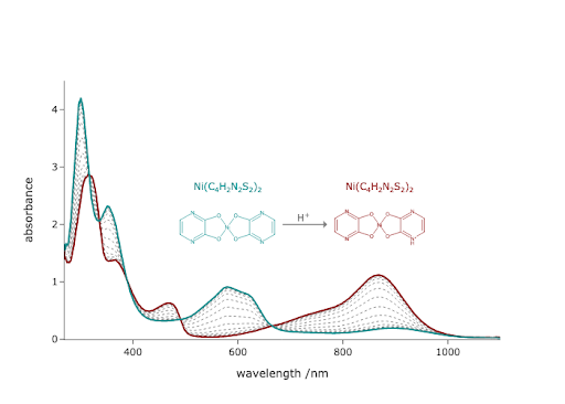

Exercise 17

Change the colors used in the final code of this chapter to ones of your choice. You should change the colors of the initial and final data, as well as the molecules being drawn. Make sure the colors for the molecules match those for the data.

import numpy as np
from plotly.subplots import make_subplots
from codechembook.quickTools import quickOpenFilenames

# First, we need the names of the files that we want to plot
# Ask the user to select the files and then sort the resulting list
data_files = quickOpenFilenames(filetypes = 'CSV files, *.csv')
sorted_data_files = sorted(data_files)

# Next, we will process one file at a time and add it to the plot
titration_series = make_subplots() # start a blank plotly figure object

# Read the data in one file and add it as a scatter trace to the figure object
for file in sorted_data_files: # loop through the data files one at a time
    # Read the data and store it in temporary x and y variables
    x_data, y_data = np.genfromtxt(file,
        delimiter = ',', skip_header = 1, unpack = True)
    
    # Add data as scatter trace with formatted lines and exclude from legend
    titration_series.add_scatter(x = x_data, y = y_data,
                                 line = dict(color = 'gray', width = 1, dash = 'dot'),
                                 name = file.stem + ' eqs', showlegend=False)

# Adjust the appearance of only the first and last traces to highlight
titration_series.update_traces(selector = 0, # specify the initial trace
    line = dict(color = 'purple', width = 2, dash = 'solid'), 
    showlegend = True, name = 'initial') 
    
titration_series.update_traces(selector = -1, # specify the final trace
    line = dict(color = 'orange', width = 2, dash = 'solid'), 
    showlegend = True, name = 'final') 

# Move the initial trace to the end of the data, so that it is drawn on top
titration_series.data = titration_series.data[1:] + titration_series.data[:1]

# Format the plot area and then show it and then save it
titration_series.update_layout(template = 'simple_white')
titration_series.update_xaxes(title = 'wavelength /nm', range = [270, 1100])
titration_series.update_yaxes(title = 'absorbance', range = [0, 4.5])

from rdkit import Chem
from rdkit.Chem import Draw
from rdkit.Chem.Draw.MolDrawing import DrawingOptions
import base64
from codechembook.symbols.TypesettingHTML import textsup

def make_mol_uri(smiles, color, bonds_wide, bonds_tall):
    '''
    Function to generate an svg of molecular drawing using rdkit and then return it in a format that is appropriate for inclusion in a Plotly figure object.

    REQUIRED PARAMETERS
    smiles (string):  Valid chemical smiles string.
    color (tuple):    Color designated in the rgb format.
    bonds_wide (int): Specifies how many bonds wide the structure is
    bonds_tall (int): Specifies how many bonds tall the structure is 

    RETURNS
    (bytes): Uri of the image for use in Plotly.
    '''
    # Create an RDKit molecule object from a SMILES string
    mol = Chem.MolFromSmiles(smiles)
    
    # Create a dictionary that defines the color of all atoms (here, the same)
    for key in range(1, 119):  # 119 is exclusive, so it goes up to 118
        DrawingOptions.elemDict[key] = color
    
    # Set options for drawing
    drawer = Draw.MolDraw2DSVG(50*bonds_wide, 50*bonds_tall) # create a canvas to draw on
    drawer.drawOptions().updateAtomPalette(DrawingOptions.elemDict) # the colors of atoms
    drawer.drawOptions().setBackgroundColour((0, 0, 0, 0)) # the canvas color
    
    # Now that the options are set, we can process the molecule drawing
    drawer.DrawMolecule(mol) # create the drawing instructions
    drawer.FinishDrawing() # use the drawing instructions to make the drawing

    # Generate the SVG instructions then convert to a Base64-encoded data URI with a Plotly-required preamble
    svg = drawer.GetDrawingText().replace('svg:', '')
    svg_data_uri = f"data:image/svg+xml;base64,{base64.b64encode(svg.encode('utf-8')).decode('utf-8')}"
    
    return svg_data_uri # return the binary code for the image
    
# Define the SMILES string for the base and acid species
base_smiles = 'C1(N=CC=N2)=C2O[Ni]3(O1)OC4=NC=CN=C4O3'
acid_smiles = '[H][N+]1=C2O[Ni]3(OC2=NC=C1)OC4=NC=CN=C4O3'

# Define colors for the base and acid species
base_color = (.5, 0, .5) # purple
acid_color = (1, 165/255, 0) # orange

# Loop through both molecules and create their respective images
for species, color, position in zip(
        [base_smiles, acid_smiles], # the SMILES strings
        [base_color, acid_color], # the colors
        [580, 870]): # the positions of the images on the plot area
    
    # Add image to plot
    titration_series.add_layout_image(
        dict(source=make_mol_uri(species, color, bonds_wide = 8, bonds_tall = 3),  
            xref='x', yref='y', # references for coordinate origin
            x=position, y=2.45, # x- and y-coordinate position of the image
            xanchor='center', yanchor='top',# alignment of image wrt x,y coords
            sizex=200, sizey=1)) # width and height of the image
        
# Add an arrow to denote the reaction
titration_series.add_annotation(
    dict(ax = 680, ay = 2, # arrow start coordinates
    x = 770, y = 2, # arrow end coordinates
    axref = 'x', ayref = 'y', xref = 'x', yref = 'y', # references for coordinates
    showarrow = True, arrowhead = 1, arrowwidth = 1.5, arrowcolor = 'grey')) # arrow format

# Add H+ label
titration_series.add_annotation(
    dict(text = 'H' + textsup('+'), font = dict(color = 'grey'),
    xref = 'x', yref = 'y', # references for coordinate origin
    x = (770+680)/2, y = 2, # x- and y-coordinate position of the image
    xanchor = 'center', yanchor = 'bottom', # location of text box wrt position
    showarrow = False))      # we want no arrow associated with this annotation

# eliminate the legend entries for all traces
titration_series.update_traces(showlegend = False)

# Now output the plot
titration_series.show('png+browser')
titration_series.write_image('titration.png', width = 6*300, height = 4*300)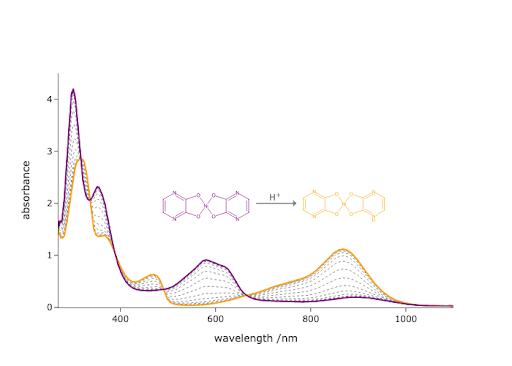

Exercise 18

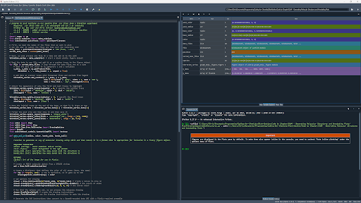
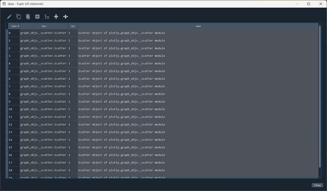
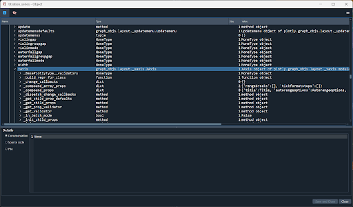
Use the Spyder variable explorer or print() to inspect the Plotly figure object created by the code in this chapter. You will find that it is structured like a dictionary. Find the keys for the following elements:

The first spectrum’s $x$-data.
The third spectrum’s $y$-data.
$x$-axis title.
The color of the line representing the last data series.

Using variable explorer