Exercises
Targeted exercises
Making ordered collections of data more flexible using list objects
Exercise 0
Make a list that contains no items.
l0 = []
print(l0)
Exercise 1
Make a list that contains, in order, the Numpy array [1, 2, 3], the string ‘frog’, and the number 3.14.
import numpy as np
l1 = [np.array([1,2,3]), 'frog', 3.14]
print(l1)
Exercise 2
Make a Numpy array with 20 elements from 0 to 10 and convert it to a list.
import numpy as np
l2 = list(np.linspace(1, 10, 20))
print(l2)
Exercise 3
Make a list that has twelve items with [1, 2, 3] repeating four times without typing in twelve numbers (i.e., use the arithmetic properties of lists).
l3 = [1,2,3]*4
print(l3)
Exercise 4
Make a list that has four items, where each item is the lists that you just made in Exercises 0-3.
l4 = [l1, l2, l3]
print(l4)
Exercise 5
Lists have a property known as \cite{mutability}, which means they can be changed after assignment (for more information see Chapter \ref{DataTypes}). In many programming languages, if you want to make a copy of list or arrays, you simply assign it to a new variable. You might make a list and assign it to the variable A, then use B = A to copy it to a new variable. Then you could change A and B independently. What happens when you do this for a list in Python?
This will produce a change to both B and A.
A = [1, 2]
B = A
B[1] = 3
print(B)
print(A)
Exercise 6
Lists have a property known as \cite{mutability}, which means they can be changed after assignment (for more information see Chapter \ref{DataTypes}). One consequence of this is that a function can change the list, and this can result in changes that are accessible outside the function. Write a function that will accept a list as an argument, and then the function replaces the first element in the list with the string "this element was changed inside a function". Make a list, print this list. Pass the list to the function, and then print the list again.
def change_list(l):
	l[0] = "this element was changed inside a function"

C = [1, 2, 3]
print(C)
change_list(C)
print(C)
Combining lists by concatenation
Exercise 7
How many items would be in the list that was made by concatenating all five lists you made in Exercises 0-4?
38. We can count them up, or we can use the len() function introduced later in this chapter to verify this. This function accepts a collection and returns the number of elements in the collection.
len(l0+l1+l2+l3+l4)Exercise 8
Repeat Exercise 3 using concatenation.
l8 = l0+l1+l2+l3
print(l9)
Exercise 9
Add the number 5 to the end of the list you made in Exercise 1.
l9 = l1 + [5]
print(l9)
Adding items to lists using the append method
Exercise 10
How many items would be in the list that was made by appending the lists you made in Exercises 1-4 onto the list made in Exercise 0?
3. The reason is that l0 starts empty, so with 0 elements. When you append l1, l2, l3 then each are appended as a list, so each is 1 element.
l0 = []
l0.append(l1)
l0.append(l2)
l0.append(l3)

print(l0)
print(len(l0))
Note: You cannot use l0.append(l1).append(l2).append(l3), because each “append” method returns the value None. This is a similar behavior to how print() also returns None. Thus, trying to chain together appends in a single line will result in trying to append l2 onto a NoneType data object, which is not possible. Try it, if you like, and you will see a type error. You will also note that we are modify the list in place.
Exercise 11
Repeat Exercises 8 & 9 using append() instead of concatenation.
l0 = []
l0.append(l1)
l0.append(l2)
l0.append(l3)

print(l0)
l1 = [np.array([1,2,3]), 'frog', 3.14]
print(l1)
l1.append(5)
print(l1)Notice that we are modifying lists in place.
Exercise 12
Sometimes it would be better to use a list, and sometimes a Numpy array. In the following cases, which do you think would be better, and why?
- You want two variables to hold the $x$ and $y$ points, respectively, of an X-ray diffraction pattern.
- Either will be fine here, but since you are likely going to want to perform math on the arrays, a Numpy array is likely better.
- You are doing a titration experiment that involves saving UV-vis spectra for each titration point, and you want to keep a record of the files that you saved, but you don’t know how many files you will need to save.
- A list is a better choice here, because the
append()method of lists is a better way to grow the collection of filenames as you make them. Though we didn’t talk about how to grow Numpy arrays, it turns out that doing so is much slower than growing lists.
- A list is a better choice here, because the
- You want a single variable to store the history of responses of a user to a code that periodically asks them to record the lab temperature.
- Similar to above, since you are going to be growing a collection, a list provides a better way to do this, via the
append()method. If you need to perform math on the collection, you can always convert it to a Numpy array when you need to.
- Similar to above, since you are going to be growing a collection, a list provides a better way to do this, via the
- You finished the experiments being discussed in this chapter and now you want to write a code that plots only the intensity of the spectrum at 450 nm (a single value) vs. the titration equivalent for each spectrum. You want to store the intensity points and titration equivalents as two separate variables for plotting.
- Either will work, though you will need to grow this collection, so a list is better choice to start. The theme here is this: if you are going to be adding to a collection, lists are faster to add to. If you want to perform math on all elements, Numpy arrays are better. You can, of course, convert from one to the other, as needed to exploit these advantages for different actions.
Determining the number of items in a collection using the len function
Exercise 13
Prove that your answer to Exercise 8 is correct, using len().
len(l0+l1+l2+l3+l4)Note: remember that lists are mutable, so if you have been running these answers in the same Python session and have been using the same variable names, you will get the wrong answer here (likely you will get 42). The reason is that the lists have changed! Exercises 10 and 11 are the culprits, which modified these lists in place. So, to get the correct answer, you might need to run the solutions to exercises 0-4 first.
Exercise 14
Starting from an empty list, create a list that goes from 0 to 4 using only append() and len()
l13 = []
l13.append(len(l13))
l13.append(len(l13))
l13.append(len(l13))
l13.append(len(l13))
l13.append(len(l13))
print(l13)
Access items in lists, arrays, or strings by indexing
Exercise 15
Create the following list and store it in a variable named data:
$[5, 1, 9, 4, 2, 8, 2, 7]$
- What is the index of the item containing 4?
- 3
- What does the \cite{expression}
data[4]yield?- 2
- Write an expression that yields the item containing the value 8.
data[-3]
- Write an expression that yields the third-to-last item in the list, and will do so, even if the length of the list changes.
data[-3]
- Replace the number 4 with the number 6.
data[3] = 6
Access subsets of lists, arrays, or strings by slicing
Exercise 16
Create a list containing ['yes', True, None, 3, 5.5, 'no']:
l15 = ['yes', True, None, 3, 5.5, 'no']:
- Write an expression that yields a subarray containing the first five items of the array.
l15[:5]
- What does the \cite{expression}
data[2:5]yield?- [None, 3, 5.5]
- Write an expression to create new list containing every other item in this list, starting with the second item.
l15[1::2]
- Write an expression to save the third through sixth items of the list as a new list stored in a variable named
data_reduced.data_reduced = l15[2:6]
- Write an expression that yields the last four items in the list and will work even if the length of the list changes (but continues to have at least 4 items).
l15[:-4]
Ordering lists and arrays by sorting
Exercise 17
Make the following list: [12, 6, 0, 2, 31, 4, 7].
- Sort this list to run in increasing order.
- Using resources outside of this book, find and use the \cite{keyword_argument} that lets you sort the same list in the reverse order. .
l16 = [12, 6, 0, 2, 31, 4, 7]
l16_sorted = sorted(l16)
print(l16_sorted)

l16_rsorted = sorted(l16, reverse = True)
print(l16_rsorted)
Obtaining a list of paths using codechembook.quickTools.quickOpenFilenames
Exercise 17
Using quickOpenFilenames(), print the paths for all the files in your downloads folder.
from codechembook.quickTools import quickOpenFilenames
print(quickOpenFilenames())
Note you will need to navigate to the downloads folder, and then select ALL files. This can be most easily done using the hot keys for this (Windows = control+a; Mac = command+a).
Exercise 18
Using the filetypes keyword argument in quickOpenFilenames(), print paths for only the pdf files in your downloads folder. If you don’t have any pdf files in your downloads folder, then download a scientific paper as a pdf, add it to your downloads and try this exercise again.
from codechembook.quickTools import quickOpenFilenames
print(quickOpenFilenames(filetypes = "*.pdf"))
The keyword will restrict all the filetypes to be only those that end in ‘.pdf’ and so you can use the same approach as above to select all the availible files.
Creating collections of objects with customized organization using dictionaries
Exercise 19
Create a dictionary in which the keys are the atomic numbers of the atoms on the second row of the periodic table, and the values are the atomic symbols.
- Write an expression to get the atomic symbol of fluorine from this dictionary.
- Write an expression to produce a string containing the formula for lithium fluoride using only this dictionary.
- Add hydrogen and helium to this dictionary .
atom_dict = {
	"3" : "Li",
	"4" : "Be",
	"5" : "B",
	"6" : "C",
	"7" : "N",
	"8" : "O",
	"9" : "F",
	"10" : "Ne",
	}

print(atom_dict["9"])
print(f"{atom_dict["3"]}{atom_dict["9"]}")

atom_dict["1"] = "H"
atom_dict["2"] = "He"

print(atom_dict)
Exercise 20
Make dictionaries of solvent properties for Benzene. Each entry of the dictionary should be a different property, and you should choose keys that have descriptive names to make it easy to remember which key goes with which property. The properties you need are:
- The IUPAC name
- The molecular weight
- The boiling point
- The density
.
benzene = {
	"IUPAC" : "benzene",
	"MW" : 78.114, #g/mol
	"BP" : 80.1, # degrees C
	"rho" : 0.8765, #g/cm3
	}

print(benzene)
Exercise 19
Repeat Exercise 20, but for the following solvents.
- Cyclohexane
- $n$-Hexane
- Toluene
- Methanol
- Acetonitrile .
cyclohexane = {
    "IUPAC": "cyclohexane",
    "MW": 84.16,       # g/mol
    "BP": 80.7,        # °C
    "rho": 0.7781,     # g/cm³
}

n_hexane = {
    "IUPAC": "hexane",
    "MW": 86.18,       # g/mol
    "BP": 68.7,        # °C
    "rho": 0.6603,     # g/cm³
}

toluene = {
    "IUPAC": "methylbenzene",
    "MW": 92.14,       # g/mol
    "BP": 110.6,       # °C
    "rho": 0.8669,     # g/cm³
}

methanol = {
    "IUPAC": "methanol",
    "MW": 32.04,       # g/mol
    "BP": 64.7,        # °C
    "rho": 0.7918,     # g/cm³
}

acetonitrile = {
    "IUPAC": "acetonitrile",
    "MW": 41.05,       # g/mol
    "BP": 81.6,        # °C
    "rho": 0.786,      # g/cm³
}
Exercise 19
Continuing from Exercise 21, create a dictionary where the keys are the names of the solvents and the values are the dictionaries that you made in Exercises 20 and 21. This means you are creating a dictionary that holds other dictionaries—a behavior known as \ul{nesting}.
solvents = {
	"benzene" : benzene,
	"cyclohexane" : cyclohexane,
	"n_hexane" : n_hexane,
	"toluene" : toluene,
	"methanol" : methanol,
	"acetonitrile" : acetonitrile,
	}

print(solvents)
Accessing information about objects using attributes
Exercise 23
Starting with the list of files in your Downloads folder that you generated in Exercise 17, sort this list and then, use the stem attribute of Path objects to print just the filename (without the extension) of the first file.
from codechembook.quickTools import quickOpenFilenames

file_list = quickOpenFilenames()
file_list = sorted(file_list)

print(file_list[0].stem)
Exercise 24
Numpy arrays also have attributes. Create a Numpy array from 0 to 5 (which includes 5) with 0.2 spacing. Using the size attribute, print the number of elements of this array.
import numpy as np
print(np.arange(0, 5.1, 0.2).size)
Performing repetitive operations using for loops
Exercise 25
Using a for loop, print each item in the list that you made in Exercise 4 on a separate line.
for item in l4:
	print(item)
Exercise 26
In Exercise 18, we found all the pdf files in your downloads folder. The output would be unwieldy. Using a for loop, place each on its own line.
from codechembook.quickTools import quickOpenFilenames

for pdffile in quickOpenFilenames(filetypes = "*.pdf"):
	print(pdffile)
Exercise 27
Suppose you have the list [3, 6, 2, 7, 5]. Using two nested for loops, print out the products of all pairs of items in the list. In other words, you will want a series of text output like: 6 x 2 = 12. Note that you should have 25 total output statements.
l27 = [3, 6, 2, 7, 5]

for i in l27:
	for j in l27:
		print(f"{i}x{j} = {i*j}")
Exercise 28
You can also iterate throuh a dictionary. When you do so, what is iterated through are the dictionary keys. Using this knowledge, print out all the solvents in the solvents dictionary.
for solvent in solvents:
	print(solvent)
Comprehensive exercises
Exercise 28
Make a single Plotly plot that shows the Maxwell-Boltzmann distribution for N$_2$ at 11 different temperatures equally spaced between $0^\circ$F and $100^\circ$F. The atmosphere is mostly nitrogen, and so these curves represent how fast the majority of molecules in the atmosphere are moving under various ’typical’ conditions.
import numpy as np
from plotly.subplots import make_subplots

# Constants
k_B = 1.380649e-23  # Boltzmann constant (J/K)
m_N2 = 28.0134e-3 / 6.02214076e23  # Mass of N2 molecule in kg (molar mass / Avogadro's number)

# Temperature range (in Kelvin)
T_min = 200  # Typical low atmospheric temperature
T_max = 400  # Typical high atmospheric temperature
T_values = np.linspace(T_min, T_max, 11)

# Speed range (in m/s)
v = np.linspace(0, 2000, 500)

# Maxwell-Boltzmann distribution function
def maxwell_boltzmann(v, T):
    factor = (m_N2 / (2 * np.pi * k_B * T)) ** (3/2)
    return 4 * np.pi * v**2 * factor * np.exp(-m_N2 * v**2 / (2 * k_B * T))

# Create figure
fig = make_subplots()

# Plot distributions for each temperature
for T in T_values:
    f_v = maxwell_boltzmann(v, T)
    fig.add_scatter(x=v, y=f_v, mode='lines', name=f'T = {T:.0f} K')

# Layout
fig.update_layout(
    title='Maxwell-Boltzmann Distribution for N₂ at Various Temperatures',
    xaxis_title='Speed (m/s)',
    yaxis_title='Probability Density',
    template='simple_white'
    )

fig.show("png")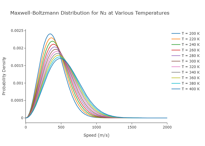
Exercise 29
Make a single Plotly plot that shows the Maxwell-Boltzmann distribution for N$_2$, O$_2$, Ar, CO$_2$, Ne, He, CH$_4$, Kr, and H$_2$ at room temperature. These are the major components of the atmosphere.
import numpy as np
from plotly.subplots import make_subplots

# Constants
k_B = 1.380649e-23  # Boltzmann constant (J/K)
Avogadro = 6.02214076e23

# Molar masses in g/mol
molar_masses = [ #list of massses in g/mol
    28.0134, #N2
    31.9988, #O2
    39.948,# Ar
    44.01, #CO2
    20.1797, #Ne
    4.0026, # He
    16.0425, # CH4
    83.798, # Kr
    2.01588 # H2
    ]

names = ["N2", "O2", "Ar", "CO2", "Ne", "He", "CH4", "Kr", "H2"]
# Convert to kg per molecule
# Room temperature in Kelvin
T = 298.15

# Speed range (in m/s)
v = np.linspace(0, 3000, 500)

# Maxwell-Boltzmann distribution function
def maxwell_boltzmann(v, T, m):
    factor = (m / (2 * np.pi * k_B * T)) ** (3/2)
    return 4 * np.pi * v**2 * factor * np.exp(-m * v**2 / (2 * k_B * T))

# Create figure
fig = make_subplots()

# Plot distributions for each gas
for i in range(len(molar_masses)):
    f_v = maxwell_boltzmann(v, T, molar_masses[i]*1e-3/Avogadro)
    fig.add_scatter(x=v, y=f_v, mode='lines', name=names[i])

# Layout
fig.update_layout(
    title='Maxwell-Boltzmann Distribution at Room Temperature (298.15 K)',
    xaxis_title='Speed (m/s)',
    yaxis_title='Probability Density',
    template='simple_white'
)

fig.show("png")
Exercise 30
Modify the final code in this chapter so that it produces a plot of each spectrum as a separate image and saves each one as a different file, all using a single for loop.
'''
A program to plot multiple uv-vis spectra from .csv files from a titration experiment
    Requires: .csv files with col 1 as wavelength and col 2 as intensity
    Written by: Ben Lear and Chris Johnson (authors@codechembook.com)
    v1.0.0 - 250131 - initial version
'''
import numpy as np
from plotly.subplots import make_subplots
from codechembook.quickTools import quickOpenFilenames

# First, we need the names of the files that we want to plot
# Ask the user to select the files and then sort the resulting list
data_files = quickOpenFilenames(filetypes = 'CSV files, *.csv')
sorted_data_files = sorted(data_files)

# Next, we will process one file at a time and add it to the plot

# Read the data in one file and add it as a scatter trace to the figure object
for file in sorted_data_files: # loop through the data files one at a time
	#going to save figures individually, so we just move the making of the figure inside the for loop
	titration_series = make_subplots() # start a blank plotly figure object
    # Read the data and store it in temporary x and y variables
    x_data, y_data = np.genfromtxt(file,
        delimiter = ',', skip_header = 1, unpack = True)

    # Add data as scatter trace with formatted lines and exclude from legend
    titration_series.add_scatter(x = x_data, y = y_data,
                                 line = dict(color = 'black', width = 2),# no need for dashed lines
                                 name = file.stem + ' eqs', showlegend=False)

	# no need to format the lines individually, since they are on separate plots

	# Format the plot area and then show it and then save it
	titration_series.update_layout(template = 'simple_white')
	titration_series.update_xaxes(title = 'wavelength /nm', range = [270, 1100])
	titration_series.update_yaxes(title = 'absorbance', range = [0, 4.5])
	titration_series.show('png+browser')
	titration_series.write_image(f'{file.stem} spectrum.png', width = 3*300, height = 2*300) # save with filename as the leading thing
Exercise 31
You now see that there are multiple properties for lines in Plotly. Let’s practice using them. You can use the online Plotly documentation or the Plotly technical chapter (Chapter \ref{ch:plotly}) to learn about other formatting. Modify the final code of this chapter to:
- Change the colors of the lines to ones that we have not yet used.
- Change the line width to a value that we have not used yet.
- Make the lines dashed, rather than solid or dotted.
- Change the font for the entire figure to ‘Courier New’
- Change the font size so that it appears roughly double the default font size.
- Change the $x$-axis range to span from 270 nm to 1000 nm. .
'''
A program to plot multiple uv-vis spectra from .csv files from a titration experiment
    Requires: .csv files with col 1 as wavelength and col 2 as intensity
    Written by: Ben Lear and Chris Johnson (authors@codechembook.com)
    v1.0.0 - 250131 - initial version
'''
import numpy as np
from plotly.subplots import make_subplots
from codechembook.quickTools import quickOpenFilenames

# First, we need the names of the files that we want to plot
# Ask the user to select the files and then sort the resulting list
data_files = quickOpenFilenames(filetypes = 'CSV files, *.csv')
sorted_data_files = sorted(data_files)

# Next, we will process one file at a time and add it to the plot
titration_series = make_subplots() # start a blank plotly figure object

# Read the data in one file and add it as a scatter trace to the figure object
for file in sorted_data_files: # loop through the data files one at a time
    # Read the data and store it in temporary x and y variables
    x_data, y_data = np.genfromtxt(file,
        delimiter = ',', skip_header = 1, unpack = True)

    # Add data as scatter trace with formatted lines and exclude from legend
    titration_series.add_scatter(x = x_data, y = y_data,
                                 line = dict(color = 'lightgray', width = 1, dash = 'dash'),
                                 name = file.stem + ' eqs', showlegend=False)

# Adjust the appearance of only the first and last traces to highlight
titration_series.update_traces(selector = 0, # specify the initial trace
    line = dict(color = 'slategrey', width = 4, dash = 'solid'),
    showlegend = True, name = 'initial')

titration_series.update_traces(selector = -1, # specify the final trace
    line = dict(color = 'link', width = 4, dash = 'solid'),
    showlegend = True, name = 'final')

# Move the initial trace to the end of the data, so that it is drawn on top
titration_series.data = titration_series.data[1:] + titration_series.data[:1]

# Format the plot area and then show it and then save it
titration_series.update_layout(template = 'simple_white', font = dict(family = "Courier New", size = 32))
titration_series.update_xaxes(title = 'wavelength /nm', range = [270, 1000])
titration_series.update_yaxes(title = 'absorbance', range = [0, 4.5])
titration_series.show('png+browser')
titration_series.write_image('titration.png', width = 3*300, height = 2*300)
In this answer, in addition to the changes with exactly specified values, we changed the color of all lines and the width of the initial and final lines, made the lines dashed.