Exercises
Exploiting built-in methods to manipulate data stored in objects
Exercise 0
Make a Numpy array that has all integers from 14 to 1, including both 1 and 14. Assign this to the variable pH. Use methods of Numpy arrays to accomplish the following (you may need to read the online Numpy documentation):
- Calculate the mean.
- Calculate the variance of the array.
- Get the standard deviation of the array.
- Sort the array so that they increase monotonically.
- Round the value of the
conc_Harray to tens digit.
import numpy as np
pH = np.array([14, 13, 12, 11, 10, 9, 8, 7, 6, 5, 4, 3, 2, 1])
a.
pH.mean()
7.5
b.
pH.var()
16.25
c.
pH.std()
4.031128874149275
d.
pH.sort()
print(pH)
[ 1 2 3 4 5 6 7 8 9 10 11 12 13 14]
e. pH.round(-1)
array([ 0, 0, 0, 0, 0, 10, 10, 10, 10, 10, 10, 10, 10, 10])
Importing subsets of libraries using from
Exercise 1
If you only want to do some math on individual values, then it may not make sense to import the whole Numpy library. Write import statements to only import the following functionality from Numpy. For example, if you wanted to import the function that is needed in order to create a Numpy array, and then make an array of the integers 1–10, assigning it to the variable x, you can use:
from numpy import array
x = array([1,2,3,4,5,6,7,8,9,10])
Following this pattern, accomplish the following:
- Import the function to compute the sine of an angle, and use it to operate on
x. - Import the function to compute the natural logarithm and use it to operate on
x. - Import the function to compute the exponential and use it to operate on
x. - Import the function to compute the square root and use it to operate on
x. .
from numpy import sin
print(sin(x))

from numpy import log
print(log(x))

from numpy import exp
print(exp(x))

from numpy import sqrt
print(sqrt(x))
Performing multiple assignment operations in one line by unpacking
Exercise 2
Pick three people you know. Using a single assignment operation assign their favorite food to a variable that is their first name.
Stanley, Shana, Ben = "peanut butter", "bread", "shrimp"Exercise 3
Define variables for the masses of hydrogen, carbon, nitrogen, and oxygen in a single line.
m_h, m_C, m_N, m_O = 1.008, 12.011, 14.007, 15.999
Exercise 4
A function that is native to Python that we have not yet seen is divmod(). Using the information returned by Python help() function, learn how to write a single line of code that will use divmod() to solve the following problem: You have a solvent bottle with 289 mL of solvent. You have a series of experiments to run that each require 7 mL of solvent. How many experiments can you run, and how much solvent will be left over. These should be assigned to separate variables. Again, use only a single line of code.
total_experiments, leftover_vol = divmod(289, 7)
print(total_experiments, leftover_vol)
Representing answers to yes/no questions using booleans
Exercise 5
Which of the following are valid values of booleans?
- True : Valid
- true : Not valid
- TRUE : Not valid
- Yes : Not valid
- yes : Not valid
- YES : Not valid
- 1 : Not valid
- 0 : Not valid
- Maybe : Not valid
Describing the location of files or folders on your computer using Pathlib
Exercise 6
Write down a statement to create a variable folder name that contains a Path object object pointing to the following folders on your computer. Use the print(<path objet>) to print the absolute path for each:
- Your Downloads folder.
- Your Documents folder.
- The folder where you are storing files for this book. This must be different from both the Downloads and Documents folder. .
from pathlib import Path
downloads = Path("C:/Users/benle/Downloads")
documents = Path("C:/Users/benle/Documents")
book = Path("C:/Users/benle/Documents/GitHub/Coding-for-Chemists/Distribution")
print(downloads)
print(documents)
print(book)
Making paths convenient and portable by specifying relative paths
Exercise 7
For the following combinations of folders, print out the relative paths that point from the first folder to the second folder. Use the relative_to() method of the Path class to find the relative path between them. You may need to use the walk_up = True keyword argument. When interpreting the results, realize that .. indicates the folder one level up from the current folder:
- From Downloads to Documents
- From Documents to Downloads
- From the folder you are using for this book to your Downloads folder
- From the folder you are using for this book to your Documents folder .
from pathlib import Path
downloads = Path("C:/Users/benle/Downloads")
documents = Path("C:/Users/benle/Documents")
book = Path("C:/Users/benle/Documents/GitHub/Coding-for-Chemists/Distribution")
print(downloads.relative_to(documents, walk_up = True))
print(documents.relative_to(downloads, walk_up = True))
print(book.relative_to(downloads, walk_up = True))
print(book.relative_to(documents, walk_up = True))
Adding codechembook to your Python installation
Exercise 8
Verify that import codechembook will run. Then use help(codechembook). How many submodules are there in this library?
7
Locating files and folders graphically with codechembook.quickTools.quickOpenFilename
Exercise 9
In this exercise, you will learn how to use quickOpenFilename() to generate a relative path from one file or folder to another file or folder.
- Use
quickOpenFilename()to select a file in your Documents folder. This will return an absolute path to the file. Assign this absolute path to a variable calledpath1. - Do the same for a file in your Downloads folder, but assign it to the variable
path2. - Use the
.relative_to()method of thePathclass to get the relative path frompath2topath1. Note you will want to use the keyword_argumentwalk_upto allow full flexibility for relative paths. .
from codechembook.quickTools import quickOpenFilename

path1 = quickOpenFilename()
path2 = quickOpenFilename()

print(path2.relative_to(path1, walk_up = True))
Exercise 10
Modern file dialogs have search features that make it so that you don’t have to click through your whole file structure to find a file or folder and get its path. Use the search feature of the file dialog in quickOpenFilename() to search for the file ‘0.999.csv’ used in this chapter and select it to get the absolute path to it. Confirm that this path exists.
from codechembook.quickTools import quickOpenFilename

print( quickOpenFilename())
You will have to run this to see it working.
Accessing data in structured text files using Numpy
Exercise 11
Use the following files supplied on \website for this exercise. Read them into Python using genfromtxt().
- Stress-Strain1.csv
- Stress-Strain1.tsv
- Stress-Strain1.ssv .
import numpy as np

csv_import = np.genfromtxt("C:/Users/benle/Documents/GitHub/CCB-HUGO/hugosite/content/Data/Stress-Strain1.csv", delimiter = ",", unpack = True, skip_header = 2)
print(csv_import)

tsv_import = np.genfromtxt("C:/Users/benle/Documents/GitHub/CCB-HUGO/hugosite/content/Data/Stress-Strain1.tsv", delimiter = "\t", unpack = True, skip_header = 2)
print(tsv_import)

ssv_import = np.genfromtxt("C:/Users/benle/Documents/GitHub/CCB-HUGO/hugosite/content/Data/Stress-Strain1.ssv", delimiter = ";", unpack = True, skip_header = 2)
print(ssv_import)
Exercise 12
Repeat Exercise 11, but only for the .csv file. Assign what is returned from genfromtxt() to a single variable. Then using this variable, unpack the values into variables that correspond to the columns in the original data file.
csv_import = np.genfromtxt("C:/Users/benle/Documents/GitHub/CCB-HUGO/hugosite/content/Data/Stress-Strain1.csv", delimiter = ",", unpack = True, skip_header = 2)
csv_col1, csv_col2 = csv_import
Exercise 13
Use genfromtxt() read the same .csv file you used in Exercise 11, but extract only the second column of data.
print(np.genfromtxt("C:/Users/benle/Documents/GitHub/CCB-HUGO/hugosite/content/Data/Stress-Strain1.csv", delimiter = ",", unpack = True, skip_header = 2, usecols = [1]))Exercise 14
As you would have noticed, the first two rows in the .csv file used in Exercise 11 contained header information. Get the information for each row, using the genfromtxt() function and setting unpack = False. You may also want to know that there are two other keyword arguments that will be useful: max_rows and dtype. The last of these specifies the type of data you are trying to read, which in this case is a string (str).
print(np.genfromtxt("C:/Users/benle/Documents/GitHub/CCB-HUGO/hugosite/content/Data/Stress-Strain1.csv", delimiter = ",", unpack = False, max_rows = 2, dtype=str))Making appealing and interactive plots using Plotly
Exercise 15
Go to the Plotly website and find an example plot. Explain how you might use that type of plot in your own research.
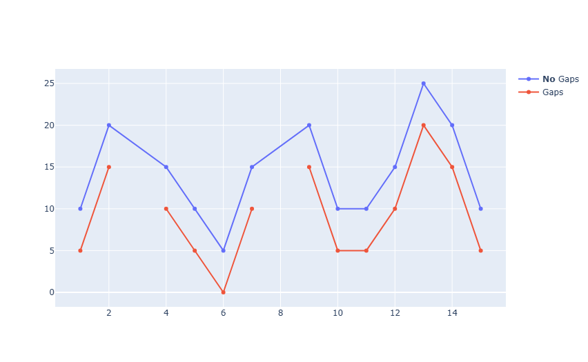 This is a line plot, often used in spectroscopy (though often without the markers).
Exercise 16
Run plotlyTest() from codechembook after importing it using from codechembook plotlyTest import plotlyTest. You can always use help(codechembook) to find this function.
from codechembook.plotlyTest import plotlyTest
plotlyTest()
Exercise 17
The plotlyTest() function you ran in Exercise 16 above should have opened a figure in your computer’s browser. One nice thing about Plotly is that these figures are interactive. Using your mouse, move your mouse cursor over the data shown. What happens? Then, click and drag your mouse to try select a region of data. What happens? Play around with this interactivity, and describe what else you find you can do.
When hovering over data points, the values are shown. When clicking and dragging, you can zoom in on a region. Double clicking on an empty space in the plot will reset the view.
Outlining your solution before coding using comments
Exercise 18
Consider the comprehensive exercises for this chapter (see below).
- Create a text outline for the solution, formatted as Python comments.
- Create a flow diagram for the solutions.
- Write a list of instructions, like you would to a human being, for how to solve them. .
# import libraries we need: numpy and plolty

# import the data file, and assign to np arrays "wavenumber" and "absorption"

# convert the absorption to % transmission

# make a plot and add a scatter of x = wavenumber and y = transmission

# show the plot as a png
Comprehensive exercises
Exercise 19
Generate Plotly plots of the following relationships:
- $e^{-x}$
- $1/x$
- $\nu_{rms}$ vs $T$ using a Maxwell-Boltzman distribution for $\ce{N2}$, over the temperature range of 200 K to 400 K
- $K_{EQ}$ as a function of $T$, for $\Delta{H}=100$ kJ$\cdot$mol$^{-1}$ and $\Delta{S}=-50$ J$\cdot$mol$^{-1}\cdot$K$^{-1}$ over the temperature range of 300 K to 400 K. .
import numpy as np
from plotly.subplots import make_subplots

x_values = np.linspace(0,10,1000)
y_values = np.exp(-1*x_values)

fig = make_subplots()
fig.add_scatter(x = x_values, y = y_values)
fig.update_xaxes(title = "x-values")
fig.update_yaxes(title = "y-values")
fig.update_layout(template = "simple_white")
fig.show("png")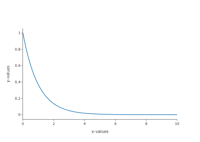
import numpy as np
from plotly.subplots import make_subplots

x_values = np.linspace(0,10,1000)
y_values = x_values**-1

fig = make_subplots()
fig.add_scatter(x = x_values, y = y_values)
fig.update_xaxes(title = "x-values")
fig.update_yaxes(title = "y-values")
fig.update_layout(template = "simple_white")
fig.show("png")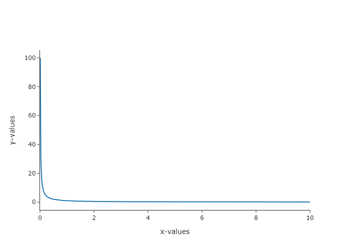
import numpy as np
from plotly.subplots import make_subplots

# --- Constants ---
R = 8.314462  # Ideal gas constant (J / (mol*K))
M_N2 = 2 * 14.007 / 1000  # Molar mass of N2 (kg/mol)

T3 = np.linspace(200, 400, 1000)  # Temperature in Kelvin (start slightly above 0)
v_rms = np.sqrt(3 * R * T3 / M_N2)

fig = make_subplots()
fig.add_scatter(x=T3, y=v_rms, mode='lines', name='v_rms (N2)')
fig.update_xaxes(title_text="Temperature / K")
fig.update_yaxes(title_text="RMS Speed")
fig.show("png")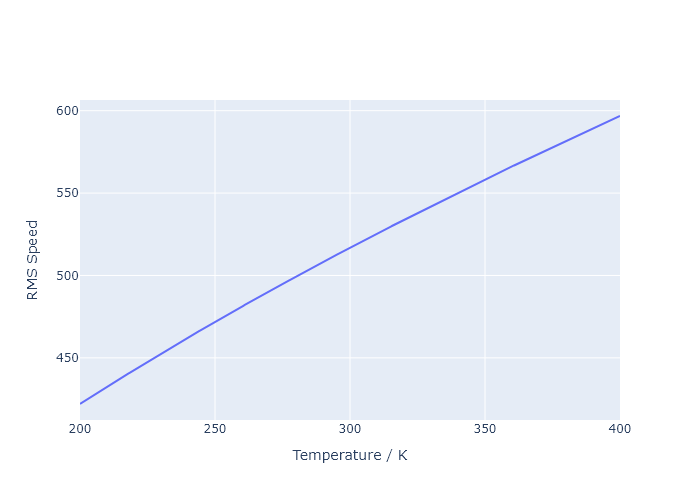
import numpy as np
from plotly.subplots import make_subplots

delta_H = -100 * 1000      # Enthalpy change (J/mol)
delta_S = 50             # Entropy change (J / (mol*K))

fig = make_subplots()
T4 = np.linspace(300, 400, 200)  # Temperature in Kelvin (avoid low T where K might explode/implode)
# Ensure no division by zero or invalid operations if T starts very low

K_EQ = np.exp(-delta_H / (R * T4) + delta_S / R)

fig.add_scatter(x=T4, y=K_EQ, mode='lines', name='K_EQ')
fig.update_xaxes(title_text="Temperature / K")
# Use log scale for K_EQ as it often spans many orders of magnitude
fig.update_yaxes(title_text="Equilibrium Constant")
fig.show("png")
Exercise 20
Consider the decay of fluorescence intensity ($I$) over time ($t$). This typically follows the functional form $I(t) = Ae^{-kt}$. Using Plotly and the values $A = 0.1$, $k = 2$:
- Plot I vs t over the range t = 0 to t = 10.
- Plot ln(I) vs t.
- Plot I vs ln(t).
- Plot ln(I) versus ln(t).
- Which of the above is the most useful, and why do you think that? .
import numpy as np
from plotly.subplots import make_subplots

t = np.linspace(0, 10, 1000)
I = 0.1*np.exp(-1*2*t)

plot = make_subplots()
plot.add_scatter(x = t, y = I)
plot.show("png")

logyplot = make_subplots()
logyplot.add_scatter(x = t, y = np.log(I))
logyplot.show("png")

logxplot = make_subplots()
logxplot.add_scatter(x = np.log(t), y =I)
logxplot.show("png")

loglogplot = make_subplots()
loglogplot.add_scatter(x = np.log(t), y =  np.log(I))
loglogplot.show("png")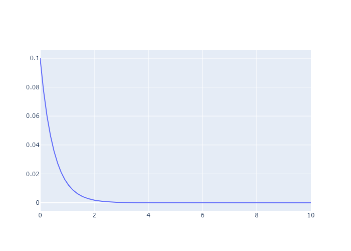

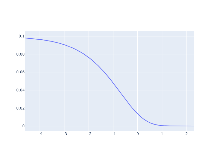

The first or second are likely the most useful. The first shows the change in real time, while the second effectively linearlizes the data.
Exercise 21
The data file ‘CO2-IR.txt’ found on the \website contains an absorption-mode FTIR spectrum of gaseous $\ce{CO2}$ with the $x$-axis in wavenumbers. Write a script to that outputs a plot of %transmission vs wavenumber. Remember that absorbance = $-\log_{10}$(transmission). Make sure you use correct axis labels! Bonus: Make the $x$-axis run from the largest to smallest numbers, which is the convention for plotting wavenumbers.
import numpy as np
from plotly.subplots import make_subplots

# import the data file, and assign to np arrays "wavenumber" and "absorption"
wavenumber, absorption  = np.genfromtxt("C:/Users/benle/Documents/GitHub/CCB-HUGO/hugosite/content/Data/CO2-IR.csv", delimiter = ",", unpack=True)

# convert the absorption to % transmission
transmission = 10**(-1* absorption)

# make a plot and add a scatter of x = wavenumber and y = transmission
fig = make_subplots()
fig.add_scatter(x = wavenumber, y = transmission)
fig.update_xaxes(title = "wavenumber /cm-1",  autorange = "reversed")
fig.update_yaxes(title = "% transmission")
fig.update_layout(template = "simple_white")

# show the plot as a png
fig.show("png")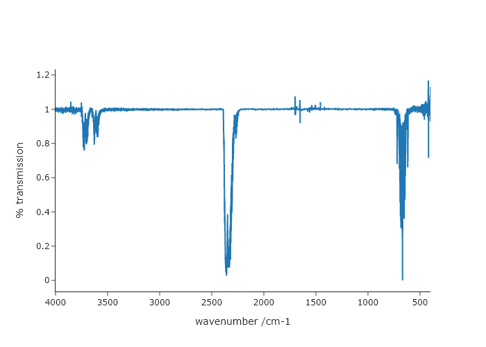
Exercise 22
Using the same file from Exercise 21 change the $x$-axis from wavenumber to wavelength (nm) and plot absorption versus wavelength. When converting between wavenumber and wavelength on the x-axis, you will need apply a Jacobian correction to the absorption. You can do this by $I(\lambda) = I(\nu) 1 \times 10^7 / \nu^2$ . Make sure you use correct axis labels!
# import libraries we need: numpy and plolty
import numpy as np
from plotly.subplots import make_subplots

# import the data file, and assign to np arrays "wavenumber" and "absorption"
wavenumber, absorption  = np.genfromtxt("C:/Users/benle/Documents/GitHub/CCB-HUGO/hugosite/content/Data/CO2-IR.csv", delimiter = ",", unpack=True)

# convert the absorption to % transmission
transmission = 10**(-1* absorption)

# make a plot and add a scatter of x = wavenumber and y = transmission
fig = make_subplots()

# convert wavenumber to wavelenth and transform absorption
wavelength = wavenumber/(10**7)
transformed_absorption = absorption*10**7/(wavenumber**2)

fig = make_subplots()
fig.add_scatter(x = wavelength, y = transformed_absorption)
fig.update_xaxes(title = "wavelength /m")
fig.update_yaxes(title = "absorption")
fig.update_layout(template = "simple_white")

# show the plot as a png
fig.show("png")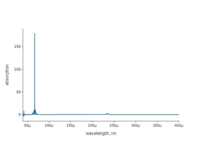
Exercise 23
One nice feature of Plotly over Matplotlib is the fact that you can change a plot after you show it and get an updated version. In Matplotlib, once you show a plot, you usually can no longer make changes and you have to start over. In the case of the final code presented in this chapter, the Plotly figure object, fig, is still in your computer’s memory and you can update it. To prove that you can do this, run the code and adjust the $x$-axis range to 450-750 nm using the range keyword of the update_xaxes() method of the figure object. Then show the plot again. Then, do the same for the $y$-axis, choosing values for range so that the resulting spectrum fills the plot area.
'''
A program to plot one uv-vis spectrum from a .csv file
    Requires: a .csv file with col 1 as wavelength and col 2 as intensity
    Written by: Ben Lear and Chris Johnson (authors@codechembook.com)
    v1.0.0 - 250131 - initial version
'''
import numpy as np # needed for genfromtxt()
from plotly.subplots import make_subplots # needed to plot
from codechembook.quickTools import quickOpenFilename

# Specify the name and place for data
data_file = quickOpenFilename()

# Import wavelength (nm) and absorbance to plot as a numpy array
x_data, y_data = np.genfromtxt(data_file,
    delimiter = ',',
    skip_header = 1,
    unpack = True)

# Construct the plot - here UVvis holds the figure object
UVvis = make_subplots() # make a figure object
UVvis.add_scatter(x = x_data, y = y_data, # make a scatter trace object
    mode = 'lines', # this ensures that we will only get lines and not markers
    showlegend = False) # this prevents a legend from being automatically created

# Format the figure
UVvis.update_yaxes(title = 'absorbance')
UVvis.update_xaxes(title = 'wavelength /nm', range = [270, 1100])
UVvis.update_layout(template = 'simple_white') # set the details for the appearance

# Display the figure
UVvis.show('browser+png') # show an interactive plot and in the spyder Plots window

# Save the spectra using the input file name but replacing .csv with the image file form
UVvis.write_image(data_file.with_suffix('.svg')) # save in the same location as the data file
UVvis.write_image(data_file.with_suffix('.png')) # save in the same location as the data file

# update the ranges...
UVvis.update_xaxes(range = [450,750])
UVvis.update_yaxes(range = [0,1])
UVvis.show("png")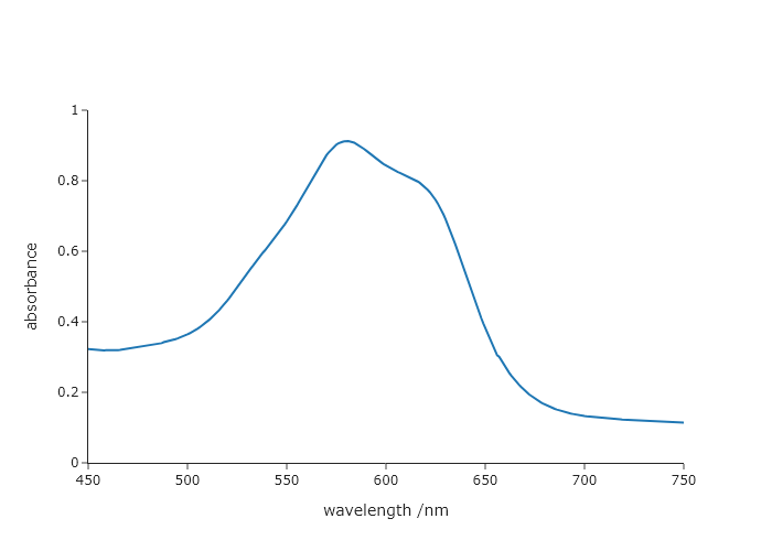
Exercise 24
In this chapter, we introduced a function that makes it easy to identify files on your computer: quickOpenFilename(). This will be nice to use when you don’t know where the file is located, or when you are choosing different files each time you run your script. However, there will be times when you simply want to use the same file over and over—for instance when you are developing and testing a code. In these cases, it can be much faster to provide the path to the file in the script. Modify the final code in this chapter, replacing the quickOpenFilename() function with a line that creates a Path object with the absolute path to the data. Verify this works, and also comment on when you might prefer this approach over the use of quickOpenFilename().
import numpy as np # needed for genfromtxt()
from plotly.subplots import make_subplots # needed to plot
from codechembook.quickTools import quickOpenFilename

# Specify the name and place for data
# data_file = quickOpenFilename()
#replace with direct path generation
from pathlib import Path
data_file = Path("C:/Users/benle/Documents/GitHub/Coding-for-Chemists/Distribution/Catalyst/Titration/UVvis/0.001.csv")

# Import wavelength (nm) and absorbance to plot as a numpy array
x_data, y_data = np.genfromtxt(data_file,
    delimiter = ',',
    skip_header = 1,
    unpack = True)

# Construct the plot - here UVvis holds the figure object
UVvis = make_subplots() # make a figure object
UVvis.add_scatter(x = x_data, y = y_data, # make a scatter trace object
    mode = 'lines', # this ensures that we will only get lines and not markers
    showlegend = False) # this prevents a legend from being automatically created

# Format the figure
UVvis.update_yaxes(title = 'absorbance')
UVvis.update_xaxes(title = 'wavelength /nm', range = [270, 1100])
UVvis.update_layout(template = 'simple_white') # set the details for the appearance

# Display the figure
UVvis.show('browser+png') # show an interactive plot and in the spyder Plots window

# Save the spectra using the input file name but replacing .csv with the image file form
UVvis.write_image(data_file.with_suffix('.svg')) # save in the same location as the data file
UVvis.write_image(data_file.with_suffix('.png')) # save in the same location as the data file
This approach will be very useful when you are documenting the workup of a particular data file, as the file is given inside the code. It is also going to be useful, when trouble shooting code, since you will not need to go through the relatively slow process of navigating to the file you want each time the code is run.