Exercises

Targeted exercises

Refactoring code to turn it into functions you can reuse

Exercise 0

Refactor the final code from Chapter 1. Create separate functions to handle the printing output, the calcPlateVols() functionality, and defining the geometry and concentrations of the well plate. The latter should take as arguments: the number of rows, the number of columns and the starting and ending concentrations and ionic strengths.

import numpy as np

# Function to generate well plate concentration matrices
def generate_wellplate_conditions(rows, cols, conc_cat, conc_HCl_start, conc_HCl_end, I_start, I_end):
    # Catalyst: constant across plate
    cat = conc_cat * np.ones((rows, cols))
    
    # HCl gradient: across columns
    MHCl_row = np.linspace(conc_HCl_start, conc_HCl_end, cols)
    MHCl_col = np.ones(rows)
    MHCl = np.outer(MHCl_col, MHCl_row)
    
    # Ionic strength gradient: across rows
    ionic_row = np.ones(cols)
    ionic_col = np.linspace(I_start, I_end, rows)
    ionic = np.outer(ionic_col, ionic_row)
    
    return cat, MHCl, ionic

# Function to calculate required stock volumes
def calculate_volumes(conc_cat, conc_HCl, I, vol_final=1.0):
    # Stock concentrations (M)
    stock_cat = 0.1
    stock_HCl = 6
    stock_NaCl = 3

    # Volume calculations (mL)
    vol_cat = conc_cat / stock_cat * vol_final
    vol_HCl = conc_HCl / stock_HCl * vol_final
    vol_NaCl = (I - conc_HCl) / stock_NaCl * vol_final
    vol_water = vol_final - vol_cat - vol_HCl - vol_NaCl

    return vol_cat, vol_HCl, vol_NaCl, vol_water

# Function to print volumes in a readable format
def print_volumes(vol_cat, vol_HCl, vol_NaCl, vol_water):
    print("[ ] Catalyst solution (mL):\n", vol_cat)
    print("[ ] HCl (mL):\n", vol_HCl)
    print("[ ] NaCl (mL):\n", vol_NaCl)
    print("[ ] Water (mL):\n", vol_water)

# === Main usage ===

# Define geometry and experimental ranges
rows, cols = 4, 6
conc_cat = 0.01
conc_HCl_start, conc_HCl_end = 0.0, 0.01
I_start, I_end = 0.02, 0.2

# Generate conditions
cat, MHCl, ionic = generate_wellplate_conditions(rows, cols, conc_cat, conc_HCl_start, conc_HCl_end, I_start, I_end)

# Calculate volumes
vol_cat, vol_HCl, vol_NaCl, vol_water = calculate_volumes(cat, MHCl, ionic)

# Output
print_volumes(vol_cat, vol_HCl, vol_NaCl, vol_water)

Exercise 0

Refactor the final code from Chapter 9. Produce a function that will automatically background subtract data passed to it. This is the refactor function.

def background_subtract(wavenumber, absorption, integration_limits):
    """Perform baseline subtraction using a linear fit between integration limits."""
    # Find nearest index to limits
    xmin_index = np.argmin(abs(wavenumber - integration_limits[0]))
    xmax_index = np.argmin(abs(wavenumber - integration_limits[1]))

    # Compute line connecting the endpoints
    m = (absorption[xmax_index] - absorption[xmin_index]) / (wavenumber[xmax_index] - wavenumber[xmin_index])
    b = absorption[xmin_index] - m * wavenumber[xmin_index]

    # Create baseline and subtract
    baseline = m * wavenumber + b
    corrected = absorption - baseline

    # Return both baseline-corrected and original baseline if needed
    return corrected, baseline

You can use it this way:

# Perform background subtraction using helper function
spec['back corr'], _ = background_subtract(spec['wavenumber'], spec['absorption'], integration_limits)

Computing derivatives using numpy.gradient

Exercise 2

For each of the following functions, determine the accuracy of a numerical derivative. Create data with an $x$-axis from 0 to $2\pi$ with 10 data points. Make a figure with two subplots, where the top plot shows the function, its analytical derivative, and its numerical derivative using the forward-backward method, and the bottom plot shows the difference between the numerical and analytical solutions.

sine
Gaussian
Lorentzian

import numpy as np
import plotly.subplots as sp
import plotly.graph_objects as go

# Set up x-axis
x = np.linspace(0, 2*np.pi, 10)
dx = x[1] - x[0]

# Forward-backward finite difference derivative
def finite_diff(y, dx):
    dydx = np.empty_like(y)
    dydx[1:-1] = (y[2:] - y[:-2]) / (2 * dx)  # central
    dydx[0] = (y[1] - y[0]) / dx              # forward
    dydx[-1] = (y[-1] - y[-2]) / dx           # backward
    return dydx

# Function definitions and derivatives
functions = {
    'sin(x)': {
        'f': np.sin(x),
        'dfdx': np.cos(x)
    },
    'Gaussian': {
        'f': np.exp(-x**2),
        'dfdx': -2*x * np.exp(-x**2)
    },
    '

Exercise 3

Starting with your code from Exercise 2 Create a plot of the root-mean-squared deviation between the numerical and analytical solutions vs. number of data points for data with 10, 20, 30, 40, and 50 points. What do you notice?

import numpy as np
import plotly.graph_objects as go

# Forward-backward finite difference
def finite_diff(y, dx):
    dydx = np.empty_like(y)
    dydx[1:-1] = (y[2:] - y[:-2]) / (2 * dx)
    dydx[0] = (y[1] - y[0]) / dx
    dydx[-1] = (y[-1] - y[-2]) / dx
    return dydx

# RMSD function
def rmsd(y1, y2):
    return np.sqrt(np.mean((y1 - y2)**2))

# Functions and their derivatives
def sin_fn(x): return np.sin(x)
def sin_deriv(x): return np.cos(x)

def gauss_fn(x): return np.exp(-x**2)
def gauss_deriv(x): return -2 * x * np.exp(-x**2)

def lorentz_fn(x): return 1 / (1 + x**2)
def lorentz_deriv(x): return -2 * x / (1 + x**2)**2

# Test point counts
N_vals = [10, 20, 30, 40, 50]

# Store RMSD results
results = {
    'sin(x)': [],
    'Gaussian': [],
    'Lorentzian': []
}

for N in N_vals:
    x = np.linspace(0, 2 * np.pi, N)
    dx = x[1] - x[0]

    # sin(x)
    y = sin_fn(x)
    dydx_num = finite_diff(y, dx)
    dydx_true = sin_deriv(x)
    results['sin(x)'].append(rmsd(dydx_num, dydx_true))

    # Gaussian
    y = gauss_fn(x)
    dydx_num = finite_diff(y, dx)
    dydx_true = gauss_deriv(x)
    results['Gaussian'].append(rmsd(dydx_num, dydx_true))

    # Lorentzian
    y = lorentz_fn(x)
    dydx_num = finite_diff(y, dx)
    dydx_true = lorentz_deriv(x)
    results['Lorentzian'].append(rmsd(dydx_num, dydx_true))

# Plot RMSD vs N
fig = go.Figure()
for label, errors in results.items():
    fig.add_scatter(x=N_vals, y=errors, mode='lines+markers', name=label)

fig.update_layout(
    title="RMSD of Numerical vs Analytical Derivative vs Number of Points",
    xaxis_title="Number of Points",
    yaxis_title="RMSD",
    yaxis_type='log'
)
fig.show()

RMSD decreases as the number of points increases — finer sampling leads to more accurate derivatives.
sin(x) tends to converge the fastest due to its smooth, periodic nature.
Gaussian and Lorentzian converge more slowly, especially the Lorentzian, which has sharp curvature and longer tails.
The improvement follows roughly power-law decay, visible as a straight line on the log scale — consistent with first-order accuracy of the forward-backward finite difference method.

Exercise 4

Redo Exercise 3 using only forward derivatives and compare the accuracy of the two methods.

import numpy as np
import plotly.graph_objects as go

# Derivative methods
def forward_diff(y, dx):
    dydx = np.empty_like(y)
    dydx[:-1] = (y[1:] - y[:-1]) / dx
    dydx[-1] = dydx[-2]  # approximate last point to match length
    return dydx

def forward_backward_diff(y, dx):
    dydx = np.empty_like(y)
    dydx[1:-1] = (y[2:] - y[:-2]) / (2 * dx)
    dydx[0] = (y[1] - y[0]) / dx
    dydx[-1] = (y[-1] - y[-2]) / dx
    return dydx

# RMSD
def rmsd(y1, y2):
    return np.sqrt(np.mean((y1 - y2)**2))

# Functions and derivatives
def sin_fn(x): return np.sin(x)
def sin_deriv(x): return np.cos(x)

def gauss_fn(x): return np.exp(-x**2)
def gauss_deriv(x): return -2 * x * np.exp(-x**2)

def lorentz_fn(x): return 1 / (1 + x**2)
def lorentz_deriv(x): return -2 * x / (1 + x**2)**2

N_vals = [10, 20, 30, 40, 50]
funcs = {
    'sin(x)': (sin_fn, sin_deriv),
    'Gaussian': (gauss_fn, gauss_deriv),
    'Lorentzian': (lorentz_fn, lorentz_deriv),
}

# Results
results_fwd = {name: [] for name in funcs}
results_fb = {name: [] for name in funcs}

# Compute RMSD for both methods
for N in N_vals:
    x = np.linspace(0, 2 * np.pi, N)
    dx = x[1] - x[0]
    
    for name, (f, df) in funcs.items():
        y = f(x)
        true = df(x)
        
        num_fwd = forward_diff(y, dx)
        num_fb = forward_backward_diff(y, dx)
        
        results_fwd[name].append(rmsd(num_fwd, true))
        results_fb[name].append(rmsd(num_fb, true))

# Plotting
fig = go.Figure()
for name in funcs:
    fig.add_scatter(x=N_vals, y=results_fwd[name], mode='lines+markers',
                    name=f'{name} (Forward)')
    fig.add_scatter(x=N_vals, y=results_fb[name], mode='lines+markers',
                    name=f'{name} (Forward-Backward)')

fig.update_layout(
    title="RMSD of Numerical Derivatives vs Number of Points",
    xaxis_title="Number of Points",
    yaxis_title="RMSD (log scale)",
    yaxis_type='log'
)
fig.show()

Forward-backward (centered) difference is more accurate, especially for smoother functions like sin(x) and the Gaussian.
The forward method converges more slowly and has consistently higher RMSD.
The advantage of central differences becomes more significant with fewer points (coarser sampling).

Importing objects from Python files in arbitrary locations

Exercise 5

Return to the final code for Chapter 7, and replace the block that imported code from an external script with code that uses importFromPy().

'''
A program to fit a titration to the Hendersson-Hassebalch equations
    Requires: pH_response from titration.py
              .csv files with col 1 as wavelength and col 2 as intensity  
    Written by: Ben Lear and Chris Johnson (authors@codechembook.com)
    v1.0.0 - 250214 - initial version
'''
import numpy as np
from pathlib import Path
from lmfit import Model
from codechembook.quickPlots import plotFit
import codechembook.symbols as cs
from codechembook.quickTools import quickOpenFilename, quickPopupMessage, importFromPy
import os

# Ask the user to specify a file with the data and read it
exp_eqs, exp_pHs = np.genfromtxt(quickOpenFilename(), delimiter = ',', skip_header = 1, unpack = True)

importFromPy("TitrationModel.py", "pH_response")

# Define a new lmfit model using the pH_response function
pH_model = Model(pH_response, independent_vars=['eqs'])  # set up the model with eqs as the 'x' axis

# Set up the fit parameter and non-adjustable parameter for initial amount of acid
pH_params = pH_model.make_params() # make a parameter object
pH_params.add('pKa', value = np.mean(exp_pHs)) # specifications for the parameter
base_i = 0.05 # the initial amount of acid

# Fit the model to the data and store the results
pH_fit = pH_model.fit(data = exp_pHs, eqs = exp_eqs, params = pH_params,  base_i = base_i)

# Create a figure for the fit result but don't show it yet
fig = plotFit(pH_fit, residual = True, xlabel = 'equivalents added', ylabel = 'pH', output = None)

# Add a horzontal line to highlight the pKa as determined by the fit
fig.add_scatter(x = [min(exp_eqs), max(exp_eqs)], 
                y = [pH_fit.params['pKa'].value, pH_fit.params['pKa'].value], 
                mode = 'lines', showlegend=False,
                line = dict(color = 'gray'))

# Add an annotation containing the best fitting pKa and its uncertainty
fig.add_annotation(x = max(exp_eqs), y = pH_fit.params['pKa'].value, 
                   xanchor = 'right', yanchor = 'bottom',
                   text = f'pKa = {pH_fit.params['pKa'].value:.3f} {cs.math.plusminus} {pH_fit.params['pKa'].stderr:.3f}',
                   showarrow = False)
fig.show('png')

Exercise 5

Using importFromPy() get the $x$ and $y$ data from the final code in Chapter 2. Then use importFromPy() to get the final extinction coefficient from the code in Chapter 5. Then make a plot of the data, but rescale the $y$ values to be in terms of concentration, rather than absorbance. Label the axes appropriately.

from codechembook.quickTools import importFromPy

# get the data from Chapter 2, take in as the figure
# don't forget you will be prompted to find the data to plot
importFromPy("PlotCatalystUVvis.py", "UVvis")


# get the extinction coefficity from chapter 5
# don't forget you will be prompted to find the folder to plot and the wavelength of interest
importFromPy("ExtinctionCalc.py", "result")

#plot the data from the UVvis figure, but with the y-rescaled
from codechembook.quickPlots import quickScatter
quickScatter(UVvis.data[0].x, UVvis.data[0].y/result.params["slope"].value, xlabel = "wavelength /nm", ylabel = "concentration /M")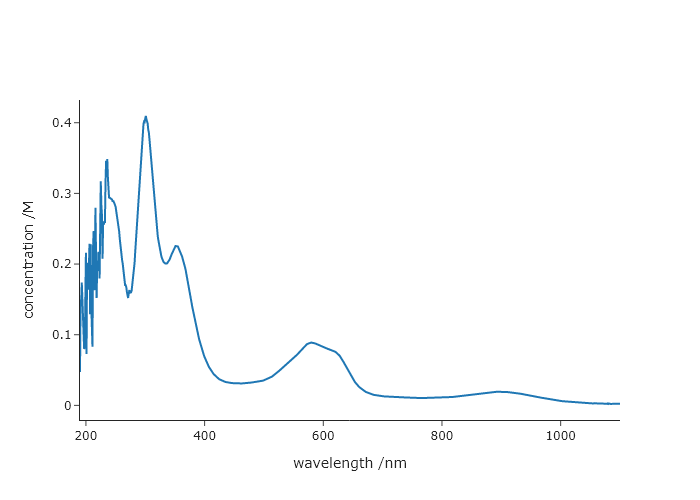

Comprehensive exercises

Exercise 7

Derivatives tend to amplify noise. Using the X-ray powder diffraction data from the website for this book, compare the results when computing the derivative first, then performing Savitzky-Golay filtering to the opposite. Which one produces more noise? You should do this in two steps, separately computing derivatives and smoothing, but note (for future use) that scipy.savgol_filter() can give you derivatives automatically with the deriv keyword.

import numpy as np
from scipy.signal import savgol_filter
from codechembook.quickTools import quickOpenFilename
from plotly.subplots import make_subplots


xrd_file = quickOpenFilename()

xrd_x, xrd_y = np.genfromtxt(xrd_file, delimiter=",", unpack = True)

fig = make_subplots(rows = 2, cols = 1)
fig.add_scatter(x = xrd_x, y = xrd_y, name = "experimental")

# compute the derivative, and then apply SG filtering
xrd_dy2 = np.gradient(xrd_y, xrd_x, edge_order = 2)
xrd_dy2_sg = savgol_filter(xrd_dy2, 5, 3)

fig.add_scatter(x = xrd_x, y = xrd_dy2_sg, name = "der then smooth", row = 2, col = 1)

# compute the sg filter, and then take the derivative
xrd_sg = savgol_filter(xrd_y, 5, 3)
xrd_sg_dy2 = np.gradient(xrd_sg, xrd_x, edge_order = 2)

fig.add_scatter(x = xrd_x, y = xrd_sg_dy2, name = "smooth, then der", row = 2, col = 1)

fig.show("browser")

Exercise 8

Write your own peak finding algorithm using derivatives. Using the file “HCl-IR.csv,” from the website for this book, which contains the FTIR spectrum of HCl, create a code that finds peaks without using scipy.find_peaks(). Remember that at a peak, the first derivative is zero and the second derivative is negative.

Read the file and plot the data, its first derivative, and its second derivative. Note that the first and second derivatives may be much smaller or larger than the data, so you may want to apply a scaling factor to each such that they are all about the same height as the data. Zoom in on a smaller peak to confirm that the derivatives look as expected.
A peak should be a maximum in the signal, a negative-going zero crossing in the first derivative, and a minimum for the second derivative. Since noise looks like peaks to a computer, you will also need to have a “threshold,” or a minimum intensity in the spectrum that distinguishes a peak from noise. Any zero crossing at a point where the signal is less than the threshold should be ignored.

The first derivative is unlikely to be precisely zero anywhere. It is much easier to find the point just before and just after the zero crossing of the first derivative and pick as the peak whichever of the two points is higher in the signal. Plot the peaks you picked on top of the data using a scatter plot. Zoomed in to a few peaks to confirm that your code works correctly.

We have also provided three other files, another FTIR spectrum “CO2-IR.csv,” and NMR spectrum “NMR.csv,: and a powder diffraction pattern “KBr.csv.: Using this same code (changing only the thresholds and scaling factors for the derivatives), find the peaks. Note that the diffraction data is noisy - comment on how does this affect your peak picker. What could you do about it?

A good trick can be to “weight” the derivatives to make it easier to tell the real peaks from the noise ones. This can be accomplished by multiplying the derivative by the signal, so that the amplitude of the derivative at each peak is enhanced. Implement this and see how this impacts your results.
You could get a more accurate estimate of the peak by explicitly determining the zero crossing. For the two points in your derivative data that are just above and just below zero, compute x value at which the derivative crosses zero. You can do this by computing the slope, $m = (y_2 - y_1)/(x_2 - x_1)$, with point 2 as the point just below zero and point 1 the point just above zero. Then, solve the same equation for $x_2$ (your zero crossing) where $y_2 = 0$ and $m$ is the slope you just computed. Implement this and comment on how it impacts your results.

import numpy as np  
from codechembook.quickPlots import quickScatter, plotFit  
from codechembook.symbols import chem  
from codechembook.quickTools import quickReadCSV  
from lmfit.models import GaussianModel, ConstantModel  
  
x, y = quickReadCSV()  
  
dydx = np.gradient(y, x)  
  
d2ydx2 = np.gradient(dydx, x)  
  
fig = quickScatter(x, y, mode = 'lines', output = 'None', name = 'Spectrum')  
fig.add_scatter(x = x, y = dydx / 10, mode = 'lines', name = 'Derivative')  
fig.add_scatter(x = x, y = d2ydx2 / 100, mode = 'lines', name = '2nd Derivative')  
fig.add_scatter(x = x, y = dydx * y, mode = 'lines', name = 'Weighted Derivative')  
fig.show('browser')  
  
  
threshold = 0.0015  
peaks = []  
for i in range(len(dydx)-1):  
    if dydx[i] >= 0 and dydx[i+1] < 0 and y[i] > threshold:  
        if y[i] >= y[i+1]:  
            peaks.append(i)  
        else:  
            peaks.append(i+1)  
  
  
fig2 = quickScatter(x, y, mode = 'lines', output = 'None', name = 'Spectrum')  
fig2.add_scatter(x = x[peaks], y = y[peaks], mode = 'markers', name = 'Peaks')  
fig2.show('browser')  
  
model = ConstantModel()  
params = model.make_params()  
for i in peaks:  
    prefix = f'G{round(x[i])}'  
    temp_model = GaussianModel(prefix = prefix)  
    pars = temp_model.make_params(amplitude = y[i], center = x[i], sigma = 0.25)  
    model = model + temp_model  
    params.update(pars)  
         
result = model.fit(y, x = x, params = params)  
  
print(result.fit_report())  
  
plotFit(result, residual = True, xlabel = f"Wavenumber ({chem.wavenumber})", ylabel = 'Intensity', output = 'png')

Exercise 9

Sometimes spectroscopists find it easier to determine the number of peaks in a complex, overlapping band, by taking the derivative of the spectrum. To figure out why, and apply this to generate initial guesses for the code at the end of Chapter 6. Hints: You can answer the fundamental question by making your own overlapping peaks and taking their derivative. Then, ask yourself what are the different ways to find peaks!

'''
Fit data to multiple gaussian components and a linear background
    Requires: a .csv file with col 1 as wavelength and col 2 as intensity  
    Written by: Ben Lear and Chris Johnson (authors@codechembook.com)
    v1.0.0 - 250207 - initial version
'''
import numpy as np
from lmfit.models import LinearModel, GaussianModel
from codechembook.quickPlots import plotFit
import codechembook.symbols as cs
from codechembook.quickTools import quickOpenFilename, quickPopupMessage
from codechembook.quickPlots import quickScatter
from plotly.subplots import make_subplots
from scipy.signal import savgol_filter, find_peaks

# Ask the user for the filename containing the data to analyze
quickPopupMessage(message = 'Select the file 0.001.csv')
file = quickOpenFilename(filetypes = 'CSV Files, *.csv')

# Read the file and unpack into arrays
wavelength, absorbance = np.genfromtxt(file, skip_header=1, unpack = True, delimiter=',')

# Set the upper and lower wavelength limits of the region of the spectrum to analyze
lowerlim, upperlim = 450, 750

# Slice data to only include the region of interest
trimmed_wavelength = wavelength[(wavelength >= lowerlim) & (wavelength < upperlim)]
trimmed_absorbance = absorbance[(wavelength >= lowerlim) & (wavelength < upperlim)]

# here is where we use derivatives and smoothing to try to identify peaks
derivative = np.gradient(trimmed_absorbance, trimmed_wavelength, edge_order=2)
smoothed_derivative = savgol_filter(derivative, 20,3)

derivative2 = np.gradient(smoothed_derivative, trimmed_wavelength, edge_order=2)
smoothed_derivative2 = savgol_filter(derivative2, 20,3)

# this part just lets us see what is happening
der_fig = make_subplots()
der_fig.add_scatter(x = trimmed_wavelength, y = trimmed_absorbance/np.max(trimmed_absorbance), name = "experimental")
der_fig.add_scatter(x = trimmed_wavelength, y = smoothed_derivative/np.max(smoothed_derivative), name = "derivative")
der_fig.add_scatter(x = trimmed_wavelength, y = smoothed_derivative2/np.max(smoothed_derivative2), name = "2nd derivative")
der_fig.show("png")

# now try to extract 3 peaks, by lowering the threshold until we find 3
i = 1
peak_indexes = []
while len(peak_indexes) != 3 and i > 0:
    peak_indexes = find_peaks(-1*smoothed_derivative2/np.max(smoothed_derivative2), prominence = i)[0]
    i = i - 0.01

position_guesses = [trimmed_wavelength[peak_indexes[0]], trimmed_wavelength[peak_indexes[1]], trimmed_wavelength[peak_indexes[2]]]

# Construct a composite model and include initial guesses
final_mod = LinearModel(prefix='lin_') # start with a linear model and add more later
pars = final_mod.guess(trimmed_absorbance, x=trimmed_wavelength) # get guesses for linear coefficients
c_guesses = position_guesses # initial guesses for centers
s_guess = 10 # initial guess for widths
a_guess = 20 # initial guess for amplitudes
for i, c in enumerate(c_guesses): # loop through each peak to add corresponding gaussian component
    gauss = GaussianModel(prefix=f'g{i+1}_') # create temporary gaussiam model
    pars.update(gauss.make_params(center=dict(value=c), # set initial guesses for parameters
                               amplitude=dict(value=a_guess, min = 0),
                               sigma=dict(value=s_guess, min = 0, max = 25)))
    final_mod = final_mod + gauss # add each peak to the overall model

# Fit the model to the data and store the results
result = final_mod.fit(trimmed_absorbance, pars, x=trimmed_wavelength)

# Create a plot of the fit results but don't show it yet
plot = plotFit(result, residual = True, components = True, xlabel = 'wavelength /nm', ylabel = 'intensity', output = None)

# Add best fitting value for the center of each gaussian component as annotations
for i in range(1, len(c_guesses)+1): # loop through components and add annotations with centers
    plot.add_annotation(text = f'{result.params[f'g{i}_center'].value:.1f} {cs.math.plusminus} {result.params[f'g{i}_center'].stderr:.1f}', 
                        x = result.params[f'g{i}_center'].value, 
                        y = i*.04 + result.params[f'g{i}_amplitude'].value / (result.params[f'g{i}_sigma'].value * np.sqrt(2*np.pi)),
                        showarrow = False)

plot.show('png') # show the final plot