Exercises

Targeted exercises

Finding local maxima using scipy.signal.find peaks

Exercise 0

Go to the the book’s website (\website) and get the following files: ‘Raman UIO66.csv, HDI IR.csv’, and ‘AuNP Raman.csv’

Using scipy.signal.find_peaks() find the peaks in these files. Experiment with the prominence, height, and width keywords to successfully only find one point per peak in each set of data. This is one potential soluton.

import numpy as np
from scipy.signal import find_peaks as fp
from codechembook.quickPlots import quickScatter as qs
#%%
Raman_file = Path("C:/Users/benle/Documents/GitHub/CCB-HUGO/hugosite/content/Data/Raman UIO66.csv")

Raman_data = np.genfromtxt(Raman_file, delimiter = ",", unpack=True)

qs(Raman_data[0], Raman_data[1])

fp(Raman_data[1], threshold = 1e4)
#%%

IR_file = Path("C:/Users/benle/Documents/GitHub/CCB-HUGO/hugosite/content/Data/HDI IR.csv")

IR_data = np.genfromtxt(IR_file, delimiter = ",", unpack=True, skip_header = 1)

qs(IR_data[0], IR_data[1])

fp(IR_data[1], prominence = 0.30)

#%%
noisey_file = Path("C:/Users/benle/Documents/GitHub/CCB-HUGO/hugosite/content/Data/AuNP Raman.csv")

noisey_data = np.genfromtxt(noisey_file, delimiter = ",", unpack=True)

qs(noisey_data[0], noisey_data[1])

fp(noisey_data[1], prominence = 1e2, width = 10)

Looping until some conditions are met with while loops

Exercise 1

Modify the final code from Chapter 5 so that it will keep asking the user for the location of the feature of interest until the user provides a valid response (something that can be converted to an integer and that is present in the $x$-data). You can simply replace the line that has the input() function with the following code

example_x, example_y = np.genfromtxt(filenames[0], unpack = True, delimiter=',', skip_header = 1)
while wavenumber = None:
	try:
		wavenumber = int(input("What is the wavelength of interest?"))
		if wavenumber in example_x:
			pass
		else:
			wavenumber = None
			print(f"Please enter a wavelength between {min(example_x)} and {max(example_x)}.")
	except
		wavenumber = None

Exercise 2

Create a game that selects a random number between 0 and 10, asks the user guess the number, and tells them if they are correct. Make sure that the user can guess the number until the user is correct. Include functionality so that it runs until you type “quit.” Also, ensure that it keeps track of the number of valid guesses.

import random

# Pick a random number between 0 and 10
target = random.randint(0, 10)

print("I'm thinking of a number between 0 and 10.")

n_guesses = 0
# Start guessing loop
while True:
    guess = input("What's your guess? ")

    # Validate input
    try:
        guess = int(guess)
        if guess > 10:
            print("Guess needs to be 10 or less!")
            continue
        if guess < 0:
            print("Guess needs to be positive!")
            continue
    except:
        if guess.lower() == "quit":
            print("Thanks for playing!")
            break
        else:
            print("Please enter an inteager.")
            continue
    n_guesses = n_guesses + 1
    if guess == target:
        print(f"🎉 Correct! You guessed it in only {n_guesses} tries!")
        break
    else:
        print(f"❌ Nope, try again.")

Exercise 3

Create a Wordle-like game that selects a random 5-letter word from a list, and then lets the user guess the word, reporting back how many letters were correct, and the position of these letters.

import random

# List of 5-letter words (you can expand this!)
word_list = ["apple", "grape", "plane", "stone", "brisk", "flame", "spine", "crane", "train", "spout"]

# Choose a random target word
target = random.choice(word_list)
print("Guess the 5-letter word!")

# Start guessing loop
while True:
    guess = input("Enter your guess: ").lower()

    if len(guess) != 5:
        print("❗ Please enter a 5-letter word.")
        continue
    if guess not in word_list:
        print("❗ That's not a valid word.")
        continue

    if guess == target:
        print("🎉 Correct! You guessed the word!")
        break

    # Track correct positions
    correct_positions = [i for i in range(5) if guess[i] == target[i]]
    correct_position_count = len(correct_positions)

    # Create copies for wrong position analysis
    target_remaining = list(target)
    guess_remaining = list(guess)

    # Remove correct-position letters to avoid double-counting
    for i in correct_positions:
        target_remaining[i] = None
        guess_remaining[i] = None

    # Count correct letters in wrong positions
    wrong_position = 0
    for g in guess_remaining:
        if g and g in target_remaining:
            wrong_position += 1
            target_remaining[target_remaining.index(g)] = None

    print(f"✅ {correct_position_count} letter(s) in the correct position.")
    if correct_positions:
        positions_str = ', '.join([str(i+1) for i in correct_positions])
        print(f"   ➤ Correct positions: {positions_str}")
    print(f"✴️ {wrong_position} correct letter(s) in the wrong position.\n")

Comprehensive exercises

Exercise 4

Often, just finding the highest point in data is not an accurate determination of the center position of a peak in a spectrum or diffraction pattern. This is especially true if your data has noise that is noticeable. In this case, it is best to use the peak finding step not as the final step, but as a way to automatically generate a reasonable initial guess for a fitting process. In the case of CV, we don’t have a great analytical function to fit the full data to, but we can fit just the area around the peak to a function like a Gaussian or parabola to get a better estimate of the true peak. Try this for the positive going and negative going peaks in the CV data presented in this chapter and see how different it is from the answer you get from find_peaks(). Another thing that happens when you fit data is that you get estimates of errors in the parameters, and so consider these as well, when comparing your results.

'''
Find the peaks of the reduction and oxidation waves in a CV experiment 
and calculate E_1/2
    Requires: CV data in a .csv file with reduction first then oxidation
    Written by: Chris Johnson and Ben Lear (authors@codechembook.com)
    v1.0.0 - 250322 - initial version
'''
import numpy as np
import scipy.signal as sps
from plotly.subplots import make_subplots
from codechembook.quickTools import quickOpenFilename, quickPopupMessage
from codechembook.symbols.greek import Delta
from codechembook.symbols.typesettingHTML import textsub, textit

# Find the data file
quickPopupMessage(message = 'Select a file with CV data.')
filename = quickOpenFilename(filetypes = 'CSV files, *.csv')
#%%
# Read the data - reduction and oxidation waves are included here
E, I = np.genfromtxt(filename, delimiter = ',', skip_header = 1, unpack = True)

# Find the index of the scan turnaround to separate the oxidation and reduction waves
i = 1 # a counter variable
stop = False # will change to true to stop the loop
while i < len(E) and stop == False: # loop until we reach the end or find the turnaround
    if E[i] < E[i-1]: # as long as E is reducing, then we are on reduction
        i += 1
    else: # E started to increase so this must be the turnaround
        stop = True
    
# Get separate arrays for reduction and oxidation
E_red, I_red = E[:i], I[:i] # reduction is simple
if E[i] == E[i+1]: # check special case where two points are the same at the turnaround
    E_ox, I_ox = E[i:], I[i:]
else: # only one point at the turnaround
    E_ox, I_ox = E[i-1:], I[i-1:] # we want to include the turnaround point too, thus i-1
                   
# Find indicies of the peak currents.  Use prominence of 10% of max to avoid noise
E_pa_index, E_pa_dict = sps.find_peaks(-1*I_red, prominence = .1*np.max(-1*I_red))
E_pc_index, E_pc_dict = sps.find_peaks(I_ox, prominence = .1*np.max(I_ox))

# Find the potentials at the peak current
E_pa = E_red[E_pa_index[0]]
E_pc = E_ox[E_pc_index[-1]]

#%% now, fit these in order to find better estimates (and errors!)
from lmfit.models import GaussianModel
from codechembook.quickPlots import quickScatter as qs

# trim the data, to only be the local area...
window_half_width = 5
local_E_red = E_red[E_pa_index[0]-window_half_width : E_pa_index[0]+window_half_width]
local_I_red = I_red[E_pa_index[0]-window_half_width : E_pa_index[0]+window_half_width]

qs(local_E_red, local_I_red)

local_E_ox = E_ox[E_pc_index[0]-window_half_width : E_pc_index[0]+window_half_width]
local_I_ox = I_ox[E_pc_index[0]-window_half_width : E_pc_index[0]+window_half_width]

qs(local_E_ox, local_I_ox)

# now fit these local regions to a gaussian...
red_gauss = GaussianModel()
red_pars = red_gauss.guess(local_I_red, x =local_E_red)
red_fit = red_gauss.fit(local_I_red, red_pars, x =local_E_red)

ox_gauss = GaussianModel()
ox_pars = ox_gauss.guess(local_I_ox, x =local_E_ox)
ox_fit = ox_gauss.fit(local_I_ox, ox_pars, x =local_E_ox)


# Print the results
print(f'E_pa = {red_fit.params["center"].value:.3f} V')
print(f'E_pc = {ox_fit.params["center"].value:.3f} V')
print(f'{Delta}E = {np.abs(red_fit.params["center"].value - ox_fit.params["center"].value):.3f} V, E1/2 = {(red_fit.params["center"].value + ox_fit.params["center"].value)*.5:.3f} V')

# Plot the results
fig = make_subplots()
fig.add_scatter(x = E_red, y = I_red, name = f'I{textsub('red')}', 
                line = dict(color = 'black'))
fig.add_scatter(x = E_ox, y = I_ox, name = f'I{textsub('ox')}', 
                line = dict(color = 'gray'))
fig.add_scatter(x = [red_fit.params["center"].value], y = red_fit.eval(x = red_fit.params["center"].value), 
                name = f'E{textsub('pa')}', mode = 'markers', 
                marker = dict(color = 'black', size = 10))
fig.add_scatter(x = [ox_fit.params["center"].value], y = ox_fit.eval(x = ox_fit.params["center"].value), 
                name = f'E{textsub('pc')}', mode = 'markers', 
                marker = dict(color = 'gray', size = 10))

# Format the plot and display
fig.update_xaxes(title = f'{textit('E')} /V', tickformat = '0.1f')
fig.update_yaxes(title = f'{textit('i')} /A')
fig.update_layout(template = 'simple_white', font_family = 'arial', 
                  font_size = 18, width = 3 * 300, height = 2 * 300, 
                  margin = dict(b = 10, t = 30, l = 10, r = 10))
fig.show('png')
fig.write_image('CVpeaks.png')

# compare peak find to fit data
print(f'''
using find_peaks: {E_pa:.3f} and {E_pc:.3f}
   using fitting: {red_fit.params["center"].value:.3f} and {ox_fit.params["center"].value:.3f}
      ''')

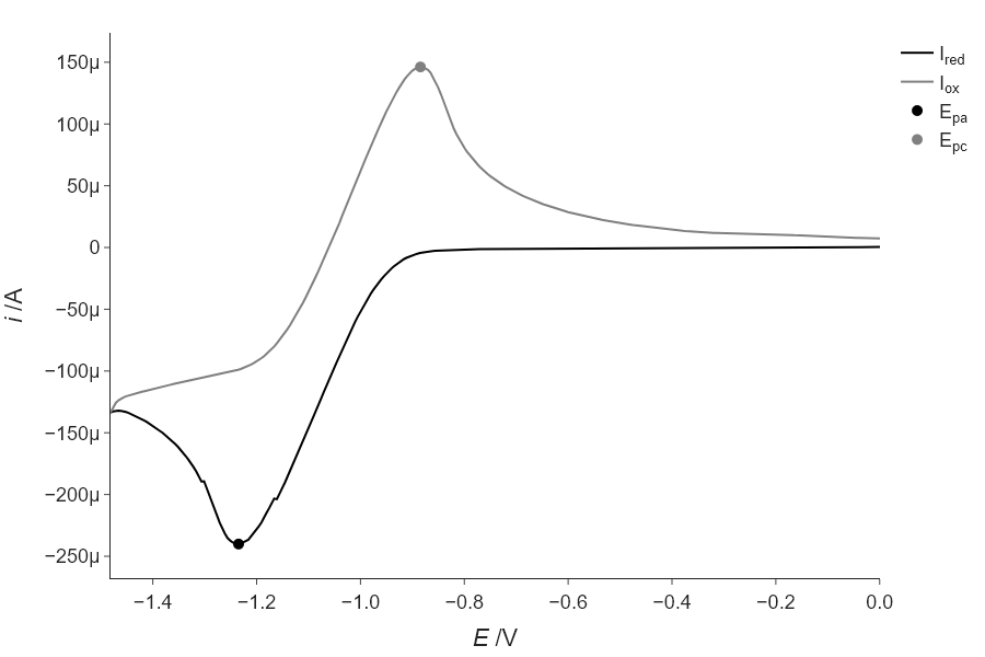
using find_peaks: -1.236 and -0.885
   using fitting: -1.235 and -0.885

Exercise 4

Modify your code above to add more noise to the data by adding normally-distributed random numbers as we did in Section \ref{Generating_noisy_test_data_using_random_numbers_from_numpy.random} and see how the difference between the find_peaks() result and the fitting result increases. Keep making the noise larger and comment on how this continues to change.

As the noise increases, the fitting approach is more robust, at just 1% noise…

'''
Find the peaks of the reduction and oxidation waves in a CV experiment 
and calculate E_1/2
    Requires: CV data in a .csv file with reduction first then oxidation
    Written by: Chris Johnson and Ben Lear (authors@codechembook.com)
    v1.0.0 - 250322 - initial version
'''
import numpy as np
import scipy.signal as sps
from plotly.subplots import make_subplots
from codechembook.quickTools import quickOpenFilename, quickPopupMessage
from codechembook.symbols.greek import Delta
from codechembook.symbols.typesettingHTML import textsub, textit

# Find the data file
quickPopupMessage(message = 'Select a file with CV data.')
filename = quickOpenFilename(filetypes = 'CSV files, *.csv')
#%%
# Read the data - reduction and oxidation waves are included here
E, I = np.genfromtxt(filename, delimiter = ',', skip_header = 1, unpack = True)

# add noise, as a fraction of the maximum value...
frac = 0.0
I = I + np.random.normal(loc = 0, scale = np.max(I)*frac, size = len(I))

# Find the index of the scan turnaround to separate the oxidation and reduction waves
i = 1 # a counter variable
stop = False # will change to true to stop the loop
while i < len(E) and stop == False: # loop until we reach the end or find the turnaround
    if E[i] < E[i-1]: # as long as E is reducing, then we are on reduction
        i += 1
    else: # E started to increase so this must be the turnaround
        stop = True
    
# Get separate arrays for reduction and oxidation
E_red, I_red = E[:i], I[:i] # reduction is simple
if E[i] == E[i+1]: # check special case where two points are the same at the turnaround
    E_ox, I_ox = E[i:], I[i:]
else: # only one point at the turnaround
    E_ox, I_ox = E[i-1:], I[i-1:] # we want to include the turnaround point too, thus i-1
                   
# Find indicies of the peak currents.  Use prominence of 10% of max to avoid noise
E_pa_index, E_pa_dict = sps.find_peaks(-1*I_red, prominence = .1*np.max(-1*I_red))
E_pc_index, E_pc_dict = sps.find_peaks(I_ox, prominence = .1*np.max(I_ox))

# Find the potentials at the peak current
E_pa = E_red[E_pa_index[0]]
E_pc = E_ox[E_pc_index[-1]]

# now, fit these in order to find better estimates (and errors!)
from lmfit.models import GaussianModel
from codechembook.quickPlots import quickScatter as qs

# trim the data, to only be the local area...
window_half_width = 5
local_E_red = E_red[E_pa_index[0]-window_half_width : E_pa_index[0]+window_half_width]
local_I_red = I_red[E_pa_index[0]-window_half_width : E_pa_index[0]+window_half_width]

qs(local_E_red, local_I_red)

local_E_ox = E_ox[E_pc_index[0]-window_half_width : E_pc_index[0]+window_half_width]
local_I_ox = I_ox[E_pc_index[0]-window_half_width : E_pc_index[0]+window_half_width]

qs(local_E_ox, local_I_ox)

# now fit these local regions to a gaussian...
red_gauss = GaussianModel()
red_pars = red_gauss.guess(local_I_red, x =local_E_red)
red_fit = red_gauss.fit(local_I_red, red_pars, x =local_E_red)

ox_gauss = GaussianModel()
ox_pars = ox_gauss.guess(local_I_ox, x =local_E_ox)
ox_fit = ox_gauss.fit(local_I_ox, ox_pars, x =local_E_ox)


# Print the results
print(f'E_pa = {red_fit.params["center"].value:.3f} V')
print(f'E_pc = {ox_fit.params["center"].value:.3f} V')
print(f'{Delta}E = {np.abs(red_fit.params["center"].value - ox_fit.params["center"].value):.3f} V, E1/2 = {(red_fit.params["center"].value + ox_fit.params["center"].value)*.5:.3f} V')

# Plot the results
fig = make_subplots()
fig.add_scatter(x = E_red, y = I_red, name = f'I{textsub('red')}', 
                line = dict(color = 'black'))
fig.add_scatter(x = E_ox, y = I_ox, name = f'I{textsub('ox')}', 
                line = dict(color = 'gray'))
fig.add_scatter(x = [red_fit.params["center"].value], y = red_fit.eval(x = red_fit.params["center"].value), 
                name = f'E{textsub('pa')}', mode = 'markers', 
                marker = dict(color = 'black', size = 10))
fig.add_scatter(x = [ox_fit.params["center"].value], y = ox_fit.eval(x = ox_fit.params["center"].value), 
                name = f'E{textsub('pc')}', mode = 'markers', 
                marker = dict(color = 'gray', size = 10))

# Format the plot and display
fig.update_xaxes(title = f'{textit('E')} /V', tickformat = '0.1f')
fig.update_yaxes(title = f'{textit('i')} /A')
fig.update_layout(template = 'simple_white', font_family = 'arial', 
                  font_size = 18, width = 3 * 300, height = 2 * 300, 
                  margin = dict(b = 10, t = 30, l = 10, r = 10))
fig.show('png')
fig.write_image('CVpeaks.png')

# compare peak find to fit data
print(f'''
using find_peaks: {E_pa:.3f} and {E_pc:.3f}
   using fitting: {red_fit.params["center"].value:.3f} and {ox_fit.params["center"].value:.3f}
      ''')

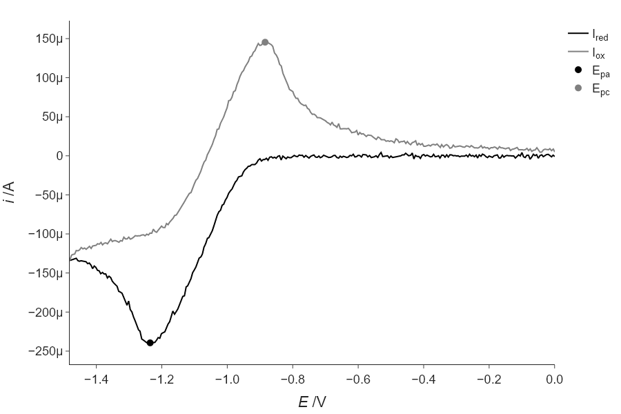
using find_peaks: -1.241 and -0.880
   using fitting: -1.236 and -0.884

Thus, the fitting is more robust (compare to the answer from above). Though your exact values may vary, as we are not using a specified seed for this random number generation.

Exercise 4

In Chapter 5, we had to ask the user which wavelength to use to extract the absorbances that we wanted to fit. Modify that code to automatically finds the peak for the initial parameter guess rather than ask the user. Note that the peak you use for the absorbances is not the highest peak in the spectrum, so you will have to get the correct peak from the list returned by find_peaks().

'''
A script to fit a calibration experiment to a line, starting wtih the UV/vis
spectra
    Requires: .csv files with col 1 as wavelength and col 2 as intensity  
               filenames should contain the concentration after an '_'
    Written by: Ben Lear and Chris Johnson (authors@codechembook.com)
    v1.0.0 - 250204 - initial version
'''
import numpy as np
from lmfit.models import LinearModel
from plotly.subplots import make_subplots
from codechembook.quickTools import quickSelectFolder, quickHTMLFormula
import codechembook.symbols as cs
    
# identify the files you wish to plot and the place you want to save them at
print('Select the folder with the calibration UVvis files.')
filenames = sorted(quickSelectFolder().glob('*csv'))

# automatically find the peak of interest
from scipy.signal import find_peaks as fp
temp_x, temp_y = np.genfromtxt(filenames[-1], unpack = True, delimiter = ",", skip_header = 1)

peak_indices = fp(temp_y, prominence = 0.5)

l_max = temp_x[peak_indices[0][-1]]

print(l_max)

# Loop through the file names, read the files, and extract the data into lists
conc, absorb = [], [] # empty lists that will hold concentrations and absorbances
for f in filenames:
    conc.append(float(f.stem.split('_')[1])) # get concentration from file name and add to list
    temp_x, temp_y = np.genfromtxt(f, unpack = True, delimiter=',', skip_header = 1) # read file
    l_max_index = np.argmin(abs(temp_x - l_max)) # Find index of x data point closest to l_max
    absorb.append(temp_y[l_max_index]) # get the closest absorbance value and add to list

# Set up and perform a linear fit to the calibration data
lin_mod = LinearModel() # create an instance of the linear model object
pars = lin_mod.guess(absorb, x=conc) # have lmfit guess at initial values
result = lin_mod.fit(absorb, pars, x=conc) # fit using these initial values
print(result.fit_report()) # print out the results of the fit

# Print out the molar absorptivity
print(f'The molar absorptivity is {result.params["slope"].value / 1:5.2f} {cs.math.plusminus} {result.params["slope"].stderr:4.2f} M{cs.typography.sup_minus}{cs.typography.sup_1}cm{cs.typography.sup_minus}{cs.typography.sup_1}')

# Construct a plot with two subplots.  Pane 1 contains the best fit and data, pane 2 the residual
fig = make_subplots(rows = 2, cols = 1) # make a blank figure object that has two subplots

# Add trace objects for the best fit, the data, and the residualto the plot
fig.add_scatter(x = result.userkws['x'], y = result.best_fit, mode = 'lines', showlegend=False, row = 1, col = 1)
fig.add_scatter(x = result.userkws['x'], y = result.data, mode = 'markers', showlegend=False, row =1, col = 1)
fig.add_scatter(x = result.userkws['x'], y = -1*result.residual, showlegend=False, row = 2, col = 1)

# Create annotation for the slope and intercept values and uncertainties as a string
annotation_string = f'''
slope = {result.params['slope'].value:.2e} {cs.math.plusminus} {result.params['slope'].stderr:.2e}<br>
intercept = {result.params['intercept'].value:.2e} {cs.math.plusminus} {result.params['intercept'].stderr:.2e}<br>
R{cs.typography.sup_2} = {result.rsquared:.3f}'''

fig.add_annotation(text = annotation_string,
                   x = np.min(result.userkws['x']), y = result.data[-1], 
                   xanchor = 'left', yanchor = 'top', align = 'left',
                   showarrow = False, )

# Create annotation for the extinction coefficient and uncertainty
fig.add_annotation(text = f'{cs.greek.epsilon} = {result.params["slope"].value:5.2f} {cs.math.plusminus} {result.params["slope"].stderr:4.2f} M<sup>-1</sup>cm<sup>-1</sup>',
                   x = np.max(result.userkws['x']), y = result.data[0], 
                   xanchor = 'right', yanchor = 'top', align = 'right',
                   showarrow = False, )

# Format the axes and the plot, then show it
fig.update_xaxes(title = 'concentration /M')
fig.update_yaxes(title = f'absorbance @ {l_max} nm', row = 1, col = 1)
fig.update_yaxes(title = 'residual absorbance', row = 2, col = 1)
fig.update_layout(template = 'simple_white', title = f'calibration for {quickHTMLFormula("(C4H2N2S2)2Ni")}')
fig.show('png')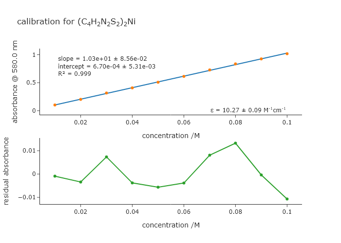

Exercise 4

Return to Exercise 6 from Chapter 8. This exercise dealt with simulating kinetics for an iodide clock. It turns out that the iodide clock only works for a narrow range of reactant concentrations, and the ones supplied there may not be the optimal ones. In this exercise, simulate the iodide clock reaction for different concentrations of B. Make the code automatically determine the amplitude of the first oscillation as a function of the concentration of B. Find the concentration for which the amplitude of this oscillation is largest. You can plot the concentration of B versus amplitude and then find the peak in this data.

import numpy as np
from scipy.integrate import solve_ivp
import plotly.graph_objects as go
from plotly.subplots import make_subplots

# === Differential Equations ===
def br_oscillator(t, y, k):
    A, B, C, D = y
    k1, k2, k3 = k
    
    dAdt = -k1 * A * B
    dBdt = k1 * A * B - k2 * B * C
    dCdt = k2 * B * C - k3 * C
    dDdt = k3 * C
    
    return [dAdt, dBdt, dCdt, dDdt]

b_concs = np.linspace(0.1, 4, 100)
A_osscilations = []
for B in b_concs:
    # === Initial conditions and parameters ===
    y0 = [10.0, B, 1.0, 0.0]        # [A], [B], [C], [D]
    k = [0.005, 0.1, 0.01]            # [k1, k2, k3]
    t_max = 10000
    t_eval = np.linspace(0, t_max, 5000)

    # === Solve ODEs ===
    sol = solve_ivp(br_oscillator, [0, t_max], y0, args=(k,), t_eval=t_eval)
    
    
    # === Analylze the ossilations
    from scipy.signal import find_peaks
    A_osscilations.append(sol.y[1][find_peaks(sol.y[1])[0][1]])
    
from codechembook.quickPlots import quickScatter
maxfit = quickScatter(b_concs, A_osscilations, xlabel = "concentration", ylabel = "peak osscilation intensity", output = None)
maxfit.add_scatter(x = [b_concs[np.argmax(A_osscilations)]], y= [A_osscilations[np.argmax(A_osscilations)]])
maxfit.show("png")

print(f"max concentration is {b_concs[np.argmax(A_osscilations)]}")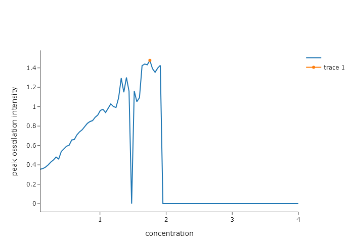

max concentration is 1.7545454545454544

Exercise 8

Using the HCl FTIR spectrum on the website for this book (HCl-spectrum.csv), find all peaks greater than 15 standard deviation above the baseline. Automatically determine the average and standard deviation for the baseline by selecting part of the data that clearly has no peaks in it.

import numpy as np
from scipy.signal import find_peaks
from plotly.subplots import make_subplots

# Load FTIR data
wavenumber, absorption = np.genfromtxt('C:/Users/benle/Documents/GitHub/CCB-HUGO/hugosite/content/Data/HCl-IR.csv', delimiter=',', unpack=True)
mask = ~np.isnan(wavenumber) & ~np.isnan(absorption)
wavenumber = wavenumber[mask]
absorption = absorption[mask]

# Step 1: Define baseline using lowest 10% of values
n_baseline_points = int(len(absorption) * 0.1)
sorted_indices = np.argsort(absorption)
baseline_region = absorption[sorted_indices[:n_baseline_points]]

# Step 2: Calculate baseline stats
baseline_avg = np.mean(baseline_region)
baseline_std = np.std(baseline_region)
threshold = baseline_avg + 15*baseline_std

# Step 3: Find peaks above threshold
peaks, properties = find_peaks(absorption, height=threshold)
peak_x = wavenumber[peaks]
peak_y = absorption[peaks]

# Step 4: Create plot using only make_subplots and add_scatter
fig = make_subplots(rows=1, cols=1, subplot_titles=["FTIR Spectrum with Peak Detection"])

# Original spectrum
fig.add_scatter(x=wavenumber, y=absorption, mode='lines', name='FTIR Spectrum', row=1, col=1)

# Threshold line
fig.add_scatter(x=[min(wavenumber), max(wavenumber)],
                y=[threshold, threshold],
                mode='lines',
                name='1σ Threshold',
                line=dict(dash='dash', color='gray'),
                row=1, col=1)

# Mark detected peaks
fig.add_scatter(x=peak_x, y=peak_y, mode='markers', name='Detected Peaks', row=1, col=1)

# Final formatting
fig.update_layout(
    title_text="Peak Detection (Absorption > 1σ above baseline)",
    width=800,
    height=400,
    showlegend=True,
    template='simple_white'
)

fig.update_xaxes(title_text="Wavenumber (cm⁻¹)", autorange='reversed')  # FTIR spectra are usually high-to-low
fig.update_yaxes(title_text="Absorbance")

fig.show('png')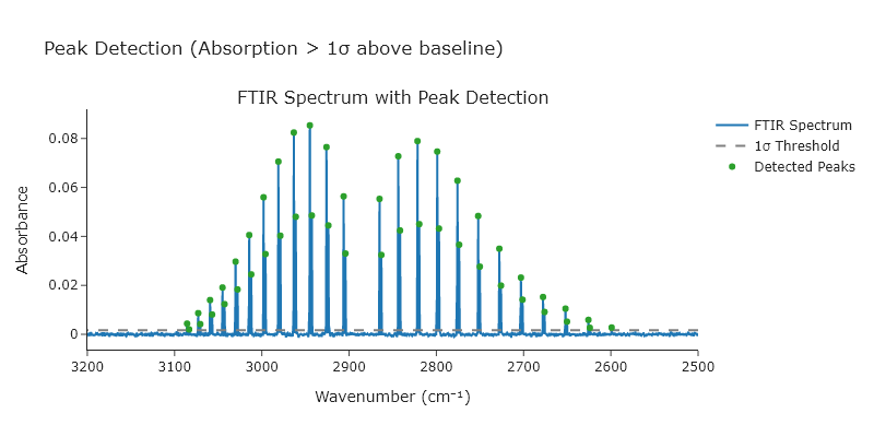

Exercise 8

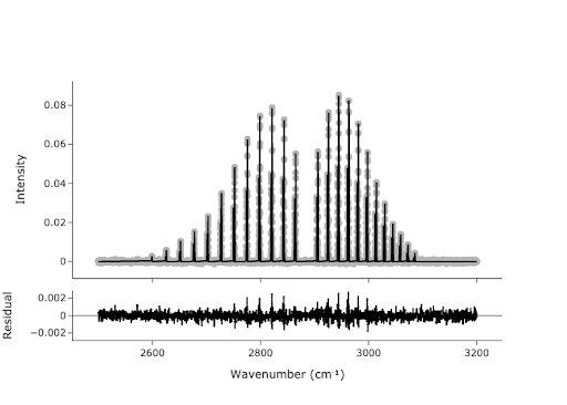
In Exercise 5, you found the peaks in the spectrum, but these points are not necessarily the values we would report for the center of each peak. We would like to get a more accurate estimate of the peak centers by fitting. We can use the peaks we found as initial guesses for our fit:

Create a model that is the sum of 47-ish Gaussians. Do not hard code the number of peaks; if the number of peaks changes, you will have to change your code. We want this to work for any number of peaks. The easiest way to do this is with a for loop.
Start with an empty model, and for each iteration, add a GaussianModel with its own prefix. At the same time, use make_params to get initial parameters for the current GaussianModel, with setting amplitude to be the $y$ value from your peak finder, center to be the $x$ value, and sigma to be something like 0.25. Hint: use the update() method for the Parameters class in LMFIT.
Plot your data initial guess to show that your initial guess is not crazy.
Now that you have the model and parameters, you should be ready to fit. Do the fitting, plot the results of the fit using plotFit(), and print the fit report. .

import numpy as np  
from scipy.signal import find_peaks  
from codechembook.quickPlots import quickScatter, plotFit  
from codechembook.symbols import chem  
from codechembook.quickTools import quickReadCSV  
from lmfit.models import GaussianModel, ConstantModel  

x, y = quickReadCSV()  
peaks, ignore = find_peaks(y, prominence=.002)  
  
fig2 = quickScatter(x, y, mode = 'lines', output = 'None', name = 'Spectrum')  
fig2.add_scatter(x = x[peaks], y = y[peaks], mode = 'markers', name = 'Peaks')  
fig2.show('browser')  
  
model = ConstantModel()  
params = model.make_params()  
for i in peaks:  
    prefix = f'G{round(x[i])}'  
    temp_model = GaussianModel(prefix = prefix)  
    pars = temp_model.make_params(amplitude = y[i], center = x[i], sigma = 0.25)  
    model = model + temp_model  
    params.update(pars)  
         
result = model.fit(y, x = x, params = params)  
  
print(result.fit_report())  
  
plotFit(result, residual = True, xlabel = f"Wavenumber ({chem.wavenumber})", ylabel = 'Intensity', output = 'browser')